预约演示
更新于:2026-07-25
Remetinostat
更新于:2026-07-25
概要
基本信息
在研机构- |
最高研发阶段终止临床2期 |
首次获批日期- |
最高研发阶段(中国)- |
特殊审评- |


登录后查看时间轴
结构/序列
分子式C16H21NO6 |
InChIKeyXDZAHHULFQIBFE-UHFFFAOYSA-N |
CAS号946150-57-8 |
关联
9
项与 Remetinostat 相关的临床试验NCT07577297
Comparative Study on the Effect of Kinesio Taping in Climacteric Women With Nonspecific Cervical Pain: ARandomized Clinical Trial.
This randomized controlled clinical trial aims to evaluate the effects of neuromuscular taping on cervical pain and health-related quality of life in climacteric women with non-specific chronic neck pain. Two taping techniques ("Y-strip" and "star-shape") will be compared with a control group receiving no intervention.
Participants will be randomly allocated to one of three groups following concealed allocation. The interventions will be applied to the cervicodorsal region (centered at C7) by an experienced physiotherapist over a 3-week period, with taping changes performed weekly. A 4-week total follow-up period will be included.
Primary and secondary outcomes will assess pain intensity, pressure pain threshold, cervical disability, cranio-cervical angle, pain perception, body satisfaction, and health-related quality of life. Measurements will be collected at baseline, weekly during the intervention, and at one-week post-intervention follow-up.
The study is designed to provide evidence on the effectiveness and feasibility of two non-invasive neuromuscular taping approaches in the management of chronic non-specific cervical pain in middle-aged women.
开始日期2026-05-20 |
申办/合作机构 |

ITMCTR2024000220
A clinical study on the treatment of knee osteoarthritis with homologous acupuncture of shape and qi
开始日期2024-09-01 |
申办/合作机构- |
NCT03875859
A Phase 2 Open Label, Single Arm Trial to Investigate the Efficacy and Safety of Topical Remetinostat Gel as Neoadjuvant Therapy in Patients Undergoing Surgical Resection of Squamous Cell Carcinoma (SCC)
The primary purpose of this study is to determine if 8 weeks of topical remetinostat applied three times daily will suppress Squamous Cell Carcinoma.
开始日期2019-12-12 |
申办/合作机构  Stanford University Stanford University [+1] |
100 项与 Remetinostat 相关的临床结果
登录后查看更多信息
100 项与 Remetinostat 相关的转化医学
登录后查看更多信息
100 项与 Remetinostat 相关的专利(医药)
登录后查看更多信息
7
项与 Remetinostat 相关的文献(医药)2024-11-01·EUROPEAN JOURNAL OF PHARMACOLOGY
Topical histone deacetylase inhibitor remetinostat improves IMQ-induced psoriatic dermatitis via suppressing dendritic cell maturation and keratinocyte differentiation and inflammation
Article
作者: Jiang, Qian ; Zhou, Xingchen ; Huang, Huining ; Jin, Liping
Psoriasis is a chronic inflammatory skin disease characterized by excessive proliferation of keratinocytes and infiltration of immune cells. Although psoriasis has entered the era of biological treatment, there is still a need to explore more effective therapeutic targets and drugs due to the presence of resistance and adverse reactions to biologics. Remetinostat, an HDAC inhibitor, can maintain its potency within the skin with minimal systemic effects, making it a promising topical medication for treating psoriasis. But its effectiveness in treating psoriasis has not been evaluated. In this study, the topical application of remetinostat significantly improved psoriasiform inflammation in an imiquimod-induced mice model by inhibiting CD86 expression of CD11C+I-A/I-E+ dendritic cells (DCs) in the skin. Moreover, remetinostat could dampen the maturation and activation of bone marrow-derived DCs in vitro, as well as the expression of psoriasis-related inflammatory mediators by keratinocytes. In addition, remetinostat could promote keratinocyte differentiation without affecting its proliferation. Our findings demonstrate that remetinostat improves psoriasis by inhibiting the maturation and activation of DCs and the differentiation and inflammation of keratinocytes, which may facilitate the potential application of remetinostat in anti-psoriasis therapy.
2024-10-01·ARCHIV DER PHARMAZIE
Soft drug inhibitors for the epigenetic targets lysine‐specific demethylase 1 and histone deacetylases
Article
作者: Baniahmad, Adina A. ; Seitz, Johannes ; Schüle, Roland ; Auth, Marina ; Preissl, Sebastian ; Hein, Lutz ; Schulz‐Fincke, Johannes ; Prinz, Tony ; Jung, Manfred ; Tzortzoglou, Pavlos ; Hau, Mirjam ; Willmann, Dominica ; Schmidtkunz, Karin ; Metzger, Eric
Abstract:
Epigenetic modulators such as lysine‐specific demethylase 1 (LSD1) and histone deacetylases (HDACs) are drug targets for cancer, neuropsychiatric disease, or inflammation, but inhibitors of these enzymes exhibit considerable side effects. For a potential local treatment with reduced systemic toxicity, we present here soft drug candidates as new LSD1 and HDAC inhibitors. A soft drug is a compound that is degraded in vivo to less active metabolites after having achieved its therapeutic function. This has been successfully applied for corticosteroids in the clinic, but soft drugs targeting epigenetic enzymes are scarce, with the HDAC inhibitor remetinostat being the only example. We have developed new methyl ester‐containing inhibitors targeting LSD1 or HDACs and compared the biological activities of these to their respective carboxylic acid cleavage products. In vitro activity assays, cellular experiments, and a stability assay identified potent HDAC and LSD1 soft drug candidates that are superior to their corresponding carboxylic acids in cellular models.
2023-06-01·Journal of labelled compounds & radiopharmaceuticals
Nitrilase mediated mild hydrolysis of a carbon‐14 nitrile for the radiosynthesis of 4‐(7‐hydroxycarbamoyl‐[1‐14C‐heptanoyl]‐oxy)‐benzoic acid methyl ester, [14C]‐SHP‐141: A novel class I/II histone deacetylase (HDAC) inhibitor
Article
作者: Moody, Thomas S. ; Chappell, Todd ; Kitson, Sean L. ; Watters, William ; Mazitschek, Ralph
A strategy has been developed for the carbon‐14 radiosynthesis of [14C]‐SHP‐141, a 4‐(7‐hydroxycarbamoyl‐heptanoyloxy)‐benzoic acid methyl ester derivative containing a terminal hydroxamic acid. The synthesis involved four radiochemical transformations. The key step in the radiosynthesis was the conversion of the 7‐[14C]‐cyano‐heptanoic acid benzyloxyamide [14C]‐4 directly into the carboxylic acid derivative, 7‐benzyloxycarbamoyl‐[14C]‐heptanoic acid [14C]‐8 using nitrilase‐113 biocatalyst. The final step involved deprotection of the benzyloxy group using catalytic hydrogenation to facilitate the release of the hydroxamic acid without cleaving the phenoxy ester. [14C]‐SHP‐141 was isolated with a radiochemical purity of 90% and a specific activity of 190 μCi/mg from four radiochemical steps starting from potassium [14C]‐cyanide in a radiochemical yield of 45%.
571
项与 Remetinostat 相关的新闻(医药)2026-07-23
*本资料仅供医疗卫生专业人士参考,请勿向非医疗卫生专业人士发放
截至07月23日15点59分,近期共有 578 本期刊发布了 968 篇文章,其中糖尿病相关的文章共 373 篇,覆盖 34 个领域的内容。中国专家参与发表的文章有 1 篇。今日,影响因子最高的文章刊登在 Journal of the American Medical Association (IF: 55.000) 期刊上。
今日头条
Headlines
01 Current obesity reports IF: 11.000 生物性别对减重手术后代谢和脂肪因子反应的影响:一项叙述性综述
Gonzalo Rivero, Amaia Rodríguez, Victoria Catalán, Beatriz Ramírez, Federico Carbone, Fabrizio Montecucco, etc.
肥胖是一种多因素、慢性、复发性非传染性疾病,以脂肪组织过度积累和代谢功能障碍为特征。越来越多的证据表明,生物性别不仅影响脂肪组织的发育和分布,还影响肥胖治疗(包括减重手术)的反应。本叙述性综述综合了当前关于减重手术后代谢结局性别差异的证据。
减重手术可诱导男性和女性显著的体重减轻和肥胖相关并发症的明显改善,但存在性别特异性的身体成分变化、脂肪组织重塑、脂肪因子分泌、炎症反应和产热适应差异。雌激素信号通过抗炎作用、改善脂肪因子谱、保留瘦体重以及刺激白色脂肪组织褐变(即白色脂肪组织中的可诱导产热脂肪细胞获得类似棕色脂肪组织的产热特性)来促进更有利的脂肪组织表型。在女性中,绝经状态是这些反应的关键生物学修饰因素。相比之下,雄激素过多与内脏脂肪堆积和胰岛素抵抗相关。
尽管主要肥胖相关并发症的缓解率在性别间大致相当,但脂肪量、激素环境和术后代谢结局的差异表明存在不同的潜在机制。虽然并发症缓解率在性别间似乎大致可比,但潜在的代谢和内分泌适应有所不同。生物性别是减重术后代谢重塑的决定因素。
本综述强调了生物性别在肥胖及其治疗中的相关性,并强调需要进行性别分层研究以阐明潜在机制,支持在肥胖管理中制定更精确、个性化的策略。
本文由 韩玉莲 编辑
扫描二维码查看源文
Current obesity reports | Volume 15, Issue 1
10.1007/s13679-026-00740-5
02 JAMA Network Open IF: 09.700 激素避孕与司美格鲁肽治疗的启动
Mille Dybdal Bager, Hannah Karin Wood-Kurland, Kathrine Kold Sørensen, Kristian Hay Kragholm, Mikkel Porsborg Andersen, Christian Torp-Pedersen, etc.
一项发表在JAMA Network Open上的全国性巢式病例对照研究,利用丹麦健康登记数据,纳入1996年至2023年间12至49岁的女性,旨在探讨激素避孕使用与后续启动司美格鲁肽治疗之间的关联。研究共识别出22,694名首次使用司美格鲁肽的女性(病例组),并按出生年份1:10匹配了229,640名未使用司美格鲁肽的对照。
结果显示,与未使用激素避孕的对照相比,所有激素避孕使用模式均与司美格鲁肽启动风险增加相关。在单一避孕类型中,校正后的风险比从复方口服片的1.42(95% CI, 1.34-1.51)到仅含孕激素宫内节育器的1.63(95% CI, 1.46-1.82)不等。在使用两种或更多避孕类型的模式中,风险比从复方口服片后使用仅含孕激素口服片的1.64(95% CI, 1.47-1.82)到其他模式的2.11(95% CI, 1.97-2.25)。校正体重指数后,关联有所减弱但未消失。
亚组分析按年龄、教育程度、收入、产次、移民状态和司美格鲁肽类型进行,结果在各亚组中基本一致。
研究结论指出,激素避孕使用与后续司美格鲁肽启动存在关联,提示需要进一步探讨女性体重管理相关因素。
本文由 韩玉莲 编辑
扫描二维码查看源文
JAMA Network Open | Volume 9, Issue 7
10.1001/jamanetworkopen.2026.24382
03 Diabetes care IF: 16.600 阿米替林、度洛西汀和普瑞巴林治疗慢性痛性糖尿病周围神经病变的随机安慰剂对照比较:对疼痛、多导睡眠图睡眠、日间功能和生活质量的影响
Julia Boyle, Malin E V Eriksson, Laura Gribble, Ravi Gouni, Sigurd Johnsen, David V Coppini, etc.
一项随机、双盲、安慰剂对照研究比较了阿米替林、度洛西汀和普瑞巴林在慢性痛性糖尿病周围神经病变患者中的疗效。研究纳入83例患者,经过8天单盲安慰剂导入期后,随机分配至三个治疗组,分别接受低剂量(14天)和高剂量(14天)药物治疗。主要终点为主观疼痛(BPI),次要终点包括多导睡眠图睡眠、日间功能和生活质量。
结果显示,三种药物均能有效减轻疼痛,但彼此之间无显著差异。在睡眠方面,普瑞巴林显著改善睡眠连续性(P<0.001),而度洛西汀增加觉醒并减少总睡眠时间(P<0.01)。度洛西汀还增强了中枢神经系统觉醒和感觉运动任务表现。普瑞巴林组的不良事件发生率显著高于其他两组(P<0.0001),主要包括疲劳、头晕和嗜睡。
研究结论认为,三种药物在镇痛效果上无显著差异,但在睡眠和日间功能等次要参数上存在差异,这些差异可能对临床治疗选择有参考价值。
本文由 韩玉莲 编辑
扫描二维码查看源文
Diabetes care | Volume 35, Issue 12
10.2337/dc12-0656
中国发表(1)
China
Cardiovascular Diabetology IF: 10.600Ahead of Print.No.01Genetically proxied glucagon-like peptide-1 and glucose-dependent insulinotropic polypeptide receptor pathway modulation is associated with favorable aging phenotypes: a drug-target Mendelian randomization study - Cardiovascular Diabetology基因代理的胰高血糖素样肽-1和葡萄糖依赖性促胰岛素多肽受体通路调节与有利的衰老表型相关:一项药物靶点孟德尔随机化研究DOI: 10.1186/s12933-026-03304-y
其他发布内容(369)
More Published Articles
J Cardiovasc Med IF: 02.000Volume 27, Issue 7No.01Triglyceride-glucose index as a predictor of adverse cardiovascular outcomes in a contemporary, diverse US population undergoing percutaneous coronary intervention甘油三酯-葡萄糖指数作为当代多样化美国人群经皮冠状动脉介入治疗后不良心血管结局的预测因子DOI: 10.2459/JCM.0000000000001916
Fundam Clin Pharmacol IF: 02.500Volume 40, Issue 4No.02When Side Effects Become Therapies: A Mechanistic Taxonomy of Adverse Drug Reactions as Translational Signals for Drug Repositioning当副作用成为疗法:药物不良反应作为药物重定位转化信号的机制分类DOI: 10.1111/fcp.70109
Yàowù shípǐn fēnxī IF: 03.000Volume 34, Issue 2No.03Can semaglutide influence tumor biomarkers? Insight from a clinical case司美格鲁肽能否影响肿瘤生物标志物?来自临床病例的见解DOI: 10.38212/2224-6614.3594
Immunobiology IF: 02.300Ahead of Print.No.04The T cell receptor associated transmembrane adaptor 1 regulates the threshold for activation of naïve human CD4+ T cellsT细胞受体相关跨膜适配器1调节人初始CD4+ T细胞活化阈值DOI: 10.1016/j.imbio.2026.153219
Journal of hazardous materials IF: 11.300Ahead of Print.No.05Pesticide exposure and all health outcomes: An umbrella review of meta-analyses of observational studies农药暴露与所有健康结局:观察性研究荟萃分析的伞状综述DOI: 10.1016/j.jhazmat.2026.143013
JACC: AdvancesAhead of Print.No.06Bidirectional Cardiorenal Interactions in Type 2 Diabetes2型糖尿病中的双向心肾相互作用DOI: 10.1016/j.jacadv.2026.103056
JACC: AdvancesAhead of Print.No.07Cardiovascular Disease Screening Programs in Low- and Middle-Income Countries: A Systematic Review中低收入国家心血管疾病筛查项目的系统综述DOI: 10.1016/j.jacadv.2026.103048
Clinical endocrinology IF: 02.400Ahead of Print.No.08The Spectrum of Congenital Hypogonadotropic Hypogonadism: A 30-Year Experience at a Tertiary Paediatric Centre先天性低促性腺激素性性腺功能减退症谱系:一家三级儿科中心30年经验DOI: 10.1111/cen.70177
Clin Exp Dermatol IF: 02.800Ahead of Print.No.09Treatment of Hailey Hailey Disease with Oral Cinacalcet: A Case Report口服西那卡塞治疗Hailey-Hailey病一例报告DOI: 10.1093/ced/llag300
Arch Endocrinol Metab IF: 02.300Volume 70, Issue 5No.10Association between triglyceride to high-density lipoprotein cholesterol ratio and new-onset diabetes mellitus甘油三酯与高密度脂蛋白胆固醇比值与新发糖尿病的关联DOI: 10.20945/2359-4292-2026-0079
Diabetes IF: 07.500Ahead of Print.No.11Deletion of 12/15-Lipoxygenase Preserves Retinal Thickness and Function and Selectively Restores Dysregulated miRNAs in Experimental Diabetes Mice敲除12/15-脂氧合酶可保护实验性糖尿病小鼠的视网膜厚度和功能并选择性恢复失调的miRNADOI: 10.2337/db26-0179
J Biochem Mol Toxicol IF: 02.800Volume 40, Issue 8No.12Investigation of the Efficacy of Orientin in Streptozotocin-Induced Type 1 Diabetes Model and Pancreatic Beta-TC6 Cells荭草苷在链脲佐菌素诱导的1型糖尿病模型及胰腺Beta-TC6细胞中的有效性研究DOI: 10.1002/jbt.71047
Yàowù shípǐn fēnxī IF: 03.000Volume 34, Issue 2No.13Advanced hybrid-green ultrasound-infrared-microwave Trifolium repens essential oil isolation with multi-target ethnomedicine bioactivity against neuropathy, inflammation and multidrug-resistant infection先进混合绿色超声-红外-微波白三叶草精油提取及其针对神经病变、炎症和多重耐药感染的多靶点民族药物生物活性DOI: 10.38212/2224-6614.3595
J Biomater Sci Polym Ed IF: 03.600Ahead of Print.No.14Integration of hydrogel forming microneedles with polyethylene glycol reservoir assisted clindamycin dermal delivery水凝胶形成微针与聚乙二醇储库联合辅助克林霉素经皮递送DOI: 10.1080/09205063.2026.2695067
ACS Appl Mater Interfaces IF: 08.200Ahead of Print.No.15Anti-Infection and Immunoregulatory Multifunctional Hydrogel for Synergistic Treatment of Diabetic Wounds抗感染与免疫调节多功能水凝胶协同治疗糖尿病伤口DOI: 10.1021/acsami.6c12616
J Bone Miner Res IF: 05.900Ahead of Print.No.16Osteoarthritis risk associated with denosumab in adults with osteoporosis: A target trial emulation骨质疏松成人使用地诺单抗相关的骨关节炎风险:一项目标试验模拟研究DOI: 10.1093/jbmr/zjag113
AJR IF: 06.100Ahead of Print.No.17Management Guidelines for Patients With Diabetes Presenting for [18F]FDG PET糖尿病患者接受[18F]FDG PET检查的管理指南DOI: 10.2214/AJR.26.35607
PloS one IF: 02.600Volume 21, Issue 7No.18Spatial and neighborhood data in the collaborative cohort of cohorts for COVID-19 Research (C4R)COVID-19研究协作队列(C4R)中的空间与邻里数据DOI: 10.1371/journal.pone.0352170
PloS one IF: 02.600Volume 21, Issue 7No.19Predictive value of complete blood cell count-based inflammatory markers for peritonitis risk in peritoneal dialysis patients: A multicenter cohort study基于全血细胞计数的炎症标志物对腹膜透析患者腹膜炎风险的预测价值:一项多中心队列研究DOI: 10.1371/journal.pone.0354120
PloS one IF: 02.600Volume 21, Issue 7No.20Protein intake and injury outcomes among fallers in the Women's Health Initiative's Objective Physical Activity and Cardiovascular Health in Older Women Study蛋白质摄入与跌倒者损伤结局:妇女健康倡议客观体力活动和心血管健康研究DOI: 10.1371/journal.pone.0353769
QJM IF: 06.400Ahead of Print.No.21The Challenge of Integrating Artificial Intelligence into Clinical Reasoning by Augmenting the Physician's Central Cognitive Role通过增强医生的核心认知角色将人工智能整合到临床推理中的挑战DOI: 10.1093/qjmed/hcag192
J Clin Endocrinol Metab IF: 05.100Ahead of Print.No.22Correction to: Sodium-Glucose Cotransporter 2 Inhibitors and New-onset Type 2 Diabetes in Adults with Prediabetes: systematic review and meta-analysis of randomized controlled trials更正:钠-葡萄糖协同转运蛋白2抑制剂与糖尿病前期成人新发2型糖尿病:随机对照试验的系统评价和荟萃分析DOI: 10.1210/clinem/dgag275
PloS one IF: 02.600Volume 21, Issue 7No.23Retraction: Application of IRSA-BP neural network in diagnosing diabetes撤稿:IRSA-BP神经网络在糖尿病诊断中的应用DOI: 10.1371/journal.pone.0354316
J Neuromuscul Dis IF: 03.400Ahead of Print.No.24Assisted leg cycle exercise for wheelchair users with muscular dystrophy辅助腿部骑行运动对肌营养不良轮椅使用者的有效性DOI: 10.1177/22143602261471196
JAMA IF: 55.000Ahead of Print.No.25Gastroparesis: A Review胃轻瘫:综述DOI: 10.1001/jama.2026.12181
Metab Syndr Relat Disord IF: 01.700Ahead of Print.No.26Extreme Temperature and Incident Diabetes Risk Among Middle-Aged and Older Adults in China: A National Longitudinal Cohort Study极端温度与中国中老年人糖尿病发病风险:一项全国纵向队列研究DOI: 10.1177/15578518261470093
Arch Endocrinol Metab IF: 02.300Volume 70, Issue 5No.27Mild and non-persistent fasting plasma glucose elevation in the first trimester of pregnancy is not associated with increased risk of gestational diabetes mellitus and adverse pregnancy outcomes妊娠早期轻度且非持续的空腹血糖升高与妊娠期糖尿病及不良妊娠结局风险增加无关DOI: 10.20945/2359-4292-2026-0077
QJM IF: 06.400Ahead of Print.No.28From Metabolic Mediation to Clinical Translation in Diabetic Kidney Disease Risk Stratification从代谢介导到临床转化:糖尿病肾病风险分层的研究进展DOI: 10.1093/qjmed/hcag193
Family practice IF: 02.200Volume 43, Issue 4No.29Pulmonary congestion assessed by lung ultrasound in stable ambulatory patients with heart failure and preserved ejection fraction in primary care初级保健中稳定门诊射血分数保留的心力衰竭患者通过肺部超声评估的肺淤血DOI: 10.1093/fampra/cmag050
Anesthesia and analgesia IF: 03.800Ahead of Print.No.30A Retrospective Propensity-Matched Cohort Study of Intravenous Versus Oral Iron Formulations for Management of Iron Deficiency Anemia in Pregnancy静脉铁剂对比口服铁剂治疗妊娠期缺铁性贫血的回顾性倾向匹配队列研究DOI: 10.1213/ANE.0000000000008229
Journal of clinical and diagnostic research IF: 00.200Volume 11, Issue 1No.31Teneligliptin in Management of Diabetic Kidney Disease: A Review of Place in Therapy特力利汀在糖尿病肾脏病治疗中的角色:治疗地位综述DOI: 10.7860/JCDR/2017/25060.9228
Int J Mol Med IF: 05.800Volume 39, Issue 4No.32A long-lasting dipeptidyl peptidase-4 inhibitor, teneligliptin, as a preventive drug for the development of hepatic steatosis in high-fructose diet-fed ob/ob mice长效二肽基肽酶-4抑制剂替格列汀作为高果糖饮食喂养的ob/ob小鼠肝脂肪变性预防药物的研究DOI: 10.3892/ijmm.2017.2899
Indian J Endocrinol MetabVolume 21, Issue 1No.33Efficacy and safety of teneligliptin替格列汀的有效性与安全性DOI: 10.4103/2230-8210.193163
Diabetes, obesity & metabolism IF: 05.700Volume 19, Issue 6No.34Efficacy and safety of canagliflozin as add-on therapy to teneligliptin in Japanese patients with type 2 diabetes mellitus: Results of a 24-week, randomized, double-blind, placebo-controlled trial卡格列净作为替格列汀附加疗法在日本2型糖尿病患者中的有效性和安全性:一项24周随机双盲安慰剂对照试验的结果DOI: 10.1111/dom.12898
J Pharmacol Sci IF: 02.900Volume 132, Issue 4No.35Changes in glucose-induced plasma active glucagon-like peptide-1 levels by co-administration of sodium-glucose cotransporter inhibitors with dipeptidyl peptidase-4 inhibitors in rodents钠-葡萄糖共转运体抑制剂与二肽基肽酶-4抑制剂联合给药对啮齿类动物葡萄糖诱导的血浆活性胰高血糖素样肽-1水平的影响DOI: 10.1016/j.jphs.2016.10.006
Diabetes Metab Syndr Obes IF: 03.000Volume 9, Issue No.36Teneligliptin real-world efficacy assessment of type 2 diabetes mellitus patients in India (TREAT-INDIA study)印度2型糖尿病患者中替格列汀的真实世界有效性评估(TREAT-INDIA研究)DOI: 10.2147/DMSO.S121770
World Journal of Cardiology IF: 02.800Volume 18, Issue 7, Page 123995-117872No.37Hearing diabetes in a one-minute electrocardiogram: Why phenotype-stratified machine learning may outperform one-size-fits-all screening在一分钟心电图中听出糖尿病:为什么表型分层机器学习可能优于一刀切筛查DOI: 10.4330/wjc.119396
J Natl Med Assoc IF: 02.300Ahead of Print.No.38Demographic and regional disparities in co-occurring diabetes and cerebrovascular disease mortality: A 24-year national retrospective analysis糖尿病与脑血管疾病共存死亡的人口学和地区差异:一项24年全国回顾性分析DOI: 10.1016/j.jnma.2026.06.007
Journal of ovarian research IF: 04.200Ahead of Print.No.39Anti-androgen therapy in polyendocrine metabolic ovary syndrome (PMOS, formerly PCOS): efficacy, safety, and phenotype-oriented clinical decision-making多内分泌代谢卵巢综合征(PMOS,原名PCOS)中的抗雄激素治疗:有效性、安全性和表型导向的临床决策DOI: 10.1186/s13048-026-02201-y
Mol Cell Biochem IF: 03.700Ahead of Print.No.40BRSK2 accumulation mediated by TRIM28 accelerates hepatocellular carcinoma progression via activating the PI3K/AKT/mTOR signaling pathwayTRIM28介导的BRSK2积累通过激活PI3K/AKT/mTOR信号通路加速肝细胞癌进展DOI: 10.1007/s11010-026-05661-4
Front Cell Neurosci IF: 04.000Volume 20, Issue No.41Up regulated hippocampal insulin pathway and oxidative stress are related to opposite changes in olfaction and episodic memory in a compensatory metabolic syndrome model in rats大鼠代偿性代谢综合征模型中上调的海马胰岛素通路和氧化应激与嗅觉和情景记忆的相反变化相关DOI: 10.3389/fncel.2026.1845387
Frontiers in endocrinology IF: 04.600Volume 17, Issue No.42Regulation of ovarian function in domestic animals: translational insights into human ovarian dynamics and dysfunction家畜卵巢功能调控:对人类卵巢动力学及功能障碍的转化见解DOI: 10.3389/fendo.2026.1863960
Frontiers in nutrition IF: 05.100Volume 13, Issue No.43Enteral nutrition-related hyperglycemia in critical illness: cascade conceptual model and implications for precision nursing-a systematic review危重症肠内营养相关高血糖:级联概念模型及对精准护理的意义——一项系统综述DOI: 10.3389/fnut.2026.1803501
Life medicineVolume 5, Issue 4No.44Connexins in metabolic control: linking brain cellular communication to systemic homeostasis连接蛋白在代谢调控中的作用:连接脑细胞通讯与全身稳态DOI: 10.1093/lifemedi/lnag018
microPublication biologyVolume 2026, Issue No.45Gene model for the ortholog of gig in Drosophila ananassaeDrosophila ananassae中gig同源基因的基因模型DOI: 10.17912/micropub.biology.001031
microPublication biologyVolume 2026, Issue No.46Gene model for the ortholog of Thor in Drosophila ananassae果蝇Drosophila ananassae中Thor同源基因的基因模型DOI: 10.17912/micropub.biology.000854
microPublication biologyVolume 2026, Issue No.47Gene model for the ortholog of Ptp61F in Drosophila ananassae果蝇Drosophila ananassae中Ptp61F直系同源基因的基因模型DOI: 10.17912/micropub.biology.001002
Pathology oncology research IF: 02.300Volume 32, Issue No.48Obesity from the perspective of the liver从肝脏视角看肥胖DOI: 10.3389/pore.2026.1612376
Frontiers in medicine IF: 03.000Volume 13, Issue No.49Population characteristics of children with short stature and construction of a predictive model for growth hormone treatment efficacy矮小症儿童人群特征及生长激素治疗有效性预测模型的构建DOI: 10.3389/fmed.2026.1818279
Zhenci yanjiuVolume 51, Issue 7No.50[Research progress on the mechanisms of electroacupuncture in the treatment of obesity]电针治疗肥胖机制的研究进展DOI: 10.13702/j.1000-0607.20251419
Zhenci yanjiuVolume 51, Issue 7No.51[Clinical study on efficacy and mechanism of separated moxibustion in the treatment of rheumatoid arthritis and related negative emotions based on gut microbiota]基于肠道菌群的隔物灸治疗类风湿关节炎及相关负面情绪的临床有效性及机制研究DOI: 10.13702/j.1000-0607.20250347
Zhenci yanjiuVolume 51, Issue 7No.52[Role of leptin receptor in the dorsal vagal complex in the inhibition of food intake in obese mice by electroacupuncture at "Zusanli" (ST36)]瘦素受体在背侧迷走复合体中介导电针“足三里”抑制肥胖小鼠摄食的作用DOI: 10.13702/j.1000-0607.20250778
Pediatrics international IF: 00.900Volume 68, Issue 1No.53ACE2/Angiotensin 1-7/Mas Receptor Axis in Thermogenic Adipose Tissue: Age-Related Implications for Pediatric Obesity产热脂肪组织中的ACE2/血管紧张素1-7/Mas受体轴:对儿童肥胖的年龄相关影响DOI: 10.1111/ped.70490
Kidney360 IF: 03.000Ahead of Print.No.54Association Between Invasive Cardiac Hemodynamics and Kidney Function in Patients with Pulmonary Hypertension肺动脉高压患者有创心脏血流动力学与肾功能的关系DOI: 10.34067/KID.0000001271
J Endocrinol Invest IF: 03.500Ahead of Print.No.55Mortality and persistence in therapy in elderly subjects with type 2 diabetes receiving gliflozins or incretins老年2型糖尿病患者接受格列净类或肠促胰素类治疗的死亡率和治疗持续性DOI: 10.1007/s40618-026-02994-1
Mol Cell Biochem IF: 03.700Ahead of Print.No.56Metabolically induced intestinal inflammation: the role of ER stress and autophagy in a porcine model of diabetes代谢诱导的肠道炎症:内质网应激和自噬在糖尿病猪模型中的作用DOI: 10.1007/s11010-026-05659-y
Int J Clin Oncol IF: 02.800Ahead of Print.No.57Identification and functional validation of lipid droplet-associated prognostic biomarkers in breast cancer via integrative multi-omics and machine learning approaches通过整合多组学和机器学习方法识别并功能验证乳腺癌中脂滴相关预后生物标志物DOI: 10.1007/s10147-026-03133-9
Acta diabetologica IF: 02.900Ahead of Print.No.58Micronutrients in immune ageing and diabetic wound healing: modulating inflammation and promoting tissue repair微量营养素在免疫衰老与糖尿病伤口愈合中的作用:调节炎症与促进组织修复DOI: 10.1007/s00592-026-02744-y
Acta diabetologica IF: 02.900Ahead of Print.No.59Improving cognition through lifestyle-induced remission of type 2 diabetes: findings from DIABEPIC-2通过生活方式干预诱导2型糖尿病缓解改善认知:DIABEPIC-2研究结果DOI: 10.1007/s00592-026-02755-9
Graefes Arch Clin Exp Ophthalmol IF: 02.300Ahead of Print.No.60Effect of cataracts on systemic factor prediction from fundus images白内障对眼底图像预测全身因素的影响DOI: 10.1007/s00417-026-07404-z
Nephrology nursing journal : IF: 00.800Volume 53, Issue 3No.61The Immeasurable Cost of the Wrong Words: When 'Noncompliance' Hid the Real Story错误言辞的不可估量代价:当“不依从”掩盖了真实故事https://pubmed.ncbi.nlm.nih.gov/42484526
European Journal of Immunology IF: 03.700Volume 56, Issue 7No.62Hematopoietic Antigen Presenting Cells Fine-Tune the Effector Phenotype of Intrathymic Unconventional αβ T Cells造血抗原呈递细胞精细调节胸腺内非常规αβ T细胞的效应表型DOI: 10.1002/eji.70243
American journal of epidemiology IF: 04.800Ahead of Print.No.63Evolving Identities or Racial Misclassification? Fluidity in race response among American Indian birthing people in Michigan and implications for public health surveillance演变中的身份还是种族分类错误?密歇根州美国印第安人分娩人群种族回答的流动性及其对公共卫生监测的影响DOI: 10.1093/aje/kwag180
JCI insight IF: 06.100Volume 11, Issue 14No.64Performance of expanded diagnostic criteria for APECED in independent cohorts and implications for earlier diagnosis扩展诊断标准在独立队列中对APECED的诊断性能及对早期诊断的意义DOI: 10.1172/jci.insight.203021
Neurosurgery IF: 03.900Ahead of Print.No.65Preoperative Opioid Weaning in Adult Spinal Deformity Surgery: Who Can Do It and Does It Predict Outcomes?成人脊柱畸形手术术前阿片类药物减量:哪些患者可以做到以及是否能预测结局?DOI: 10.1227/neu.0000000000004174
Biomedical chromatography IF: 01.700Volume 40, Issue 9No.66Integrated GNPS Molecular Networking and Network Pharmacology Uncover Methylophiopogonanone B as a Novel Anti-Inflammatory Agent From Polygonatum cyrtonema Hua Targeting the SRC-PI3K-Akt Pathway整合GNPS分子网络与网络药理学揭示甲基麦冬黄烷酮B作为来自多花黄精的新型抗炎剂靶向SRC-PI3K-Akt通路DOI: 10.1002/bmc.70570
Clinical spine surgery IF: 01.700Ahead of Print.No.67The Impact of Central and Foraminal Stenosis Severity on the Need for Surgery After Epidural Steroid Injection中央型和椎间孔型狭窄严重程度对硬膜外类固醇注射后手术需求的影响DOI: 10.1097/BSD.0000000000002047
Expert Rev Endocrinol Metab IF: 02.800Ahead of Print.No.68Do women with young-onset type 2 diabetes have a higher risk for adverse pregnancy outcomes?年轻发病的2型糖尿病女性是否面临更高的不良妊娠结局风险?DOI: 10.1080/17446651.2026.2707297
Omics : IF: 01.600Ahead of Print.No.69Multi-Omics Evidence from Genetics Reveals an Association between the Hypoglycemic Drug Target DPP4 and Primary Ovarian Failure遗传学多组学证据揭示降糖药物靶点DPP4与原发性卵巢功能不全的关联DOI: 10.1177/15578100261467515
JCRPE IF: 01.500Ahead of Print.No.70Off-Label Use of Teriparatide for Osteotomy Healing in an Adolescent with Osteogenesis Imperfecta Type VIII: A Case Report特立帕肽超说明书用于成骨不全症VIII型青少年截骨愈合的病例报告DOI: 10.4274/jcrpe.galenos.2026.2026-3-21
Journal of materials chemistry IF: 05.700Ahead of Print.No.71Peptide-coordinated silver nanoassemblies: a multifunctional hydrogel platform for infected diabetic wound healing肽配位银纳米组装体:用于感染性糖尿病伤口愈合的多功能水凝胶平台DOI: 10.1039/d6tb00694a
Current diabetes reviews IF: 01.900Ahead of Print.No.72Advancing Diabetes Treatment Through NanoPhytotherapeutics: Uncovering the Therapeutic Promise of Syzygium Cumini, Pterocarpus Santalinus, and Momordica Cymbalaria通过纳米植物疗法推进糖尿病治疗:揭示蒲桃、紫檀和木鳖果的治疗前景DOI: 10.2174/0115733998470934260630070603
Mini Rev Med Chem IF: 03.300Ahead of Print.No.73Computational Drug Repurposing: Exploring New Uses for Existing Molecules in the Treatment of Diabetes Mellitus计算药物重定位:探索现有分子在糖尿病治疗中的新用途DOI: 10.2174/0113895575439810260513062337
Diabetes, obesity & metabolism IF: 05.700Ahead of Print.No.74Closer Association of Liver Stiffness Than Liver Fat Content With Imaging-Derived Neurovascular Coupling in a Metabolic Dysfunction-Associated Steatotic Liver Disease Cohort在代谢功能障碍相关脂肪性肝病队列中,肝脏硬度与影像学衍生的神经血管耦合的关联比肝脏脂肪含量更密切DOI: 10.1111/dom.71125
Diabetes, obesity & metabolism IF: 05.700Ahead of Print.No.75Association Between Time in Range and Advanced Cardiovascular-Kidney-Metabolic Syndrome in Older Adults With Type 2 Diabetes老年2型糖尿病患者葡萄糖目标范围内时间与晚期心血管-肾脏-代谢综合征的关联DOI: 10.1111/dom.71143
Diabetes, obesity & metabolism IF: 05.700Ahead of Print.No.76Joint Trajectories of Physical Activity and Depressive Symptoms and Incident Cardiometabolic Multimorbidity: A Multi-Cohort Study体力活动与抑郁症状的联合轨迹及新发心血管代谢多病共存:一项多队列研究DOI: 10.1111/dom.71115
J Clin Transl Hepatol IF: 04.200Volume 14, Issue 6No.77Reducing the Risk of Overt Hepatic Encephalopathy Recurrence: A Narrative Review降低显性肝性脑病复发风险:一项叙述性综述DOI: 10.14218/JCTH.2025.00698
Small scienceVolume 6, Issue 7No.78Upconverting Nanoparticles for Bimodal Luminescence and Magnetic Resonance Imaging of Langerhans Islets上转换纳米颗粒用于朗格汉斯岛双模态发光和磁共振成像DOI: 10.1002/smsc.70344
Frontiers in nutrition IF: 05.100Volume 13, Issue No.79Dysregulation of phosphatidylethanolamine metabolism associated with upregulation of PNPLA6 in high-fat diet/streptozotocin mice高脂饮食/链脲佐菌素小鼠中磷脂酰乙醇胺代谢失调与PNPLA6上调相关DOI: 10.3389/fnut.2026.1799991
Front Rehabil Sci IF: 01.900Volume 7, Issue No.80Clinical and psychological adjustment to prosthesis use in lower-limb amputees: focus on differences between traditional and high-technology rehabilitation下肢截肢者假肢使用的临床与心理适应:传统与高科技康复的差异DOI: 10.3389/fresc.2026.1830110
Przegl?d Gastroenterologiczny IF: 02.500Volume 21, Issue 2No.81The prevalence of exocrine pancreatic insufficiency in diabetes mellitus - a multicentre study糖尿病中外分泌胰腺功能不全的患病率——一项多中心研究DOI: 10.5114/pg.2026.161673
FCVM IF: 02.900Volume 13, Issue No.82Prognostic significance of pan-immune-inflammatory value in adverse cardiovascular and cerebrovascular events post-percutaneous coronary intervention in diabetic patients with coronary heart disease泛免疫炎症值对糖尿病冠心病患者经皮冠状动脉介入术后不良心脑血管事件的预后意义DOI: 10.3389/fcvm.2026.1750706
J Family Med Prim Care IF: 01.000Volume 15, Issue 5No.83Uptake of influenza and pneumococcal vaccines among older adults attending primary health care centers in Riyadh, Saudi Arabia沙特阿拉伯利雅得初级卫生保健中心老年人流感和肺炎球菌疫苗接种率研究DOI: 10.4103/jfmpc.jfmpc_396_26
J Phys Chem C Nanomater Interfaces IF: 03.200Volume 130, Issue 28No.84Electronic Structure Engineering of Cu-Mn Spinel Oxides via Ni Substitution for Enhanced Electrocatalytic Glucose Oxidation通过镍取代调控铜锰尖晶石氧化物的电子结构以增强电催化葡萄糖氧化DOI: 10.1021/acs.jpcc.6c03237
Cell press blueVolume 1, Issue 4No.85NodoMap: A single-cell and spatial transcriptomic atlas of the mouse nodose ganglionNodoMap:小鼠结状神经节单细胞和空间转录组图谱DOI: 10.1016/j.cpblue.2026.100072
JCEM case reportsVolume 4, Issue 8No.86Autosomal dominant hypophosphatemic rickets caused by a novel pathogenic variant in FGF23新型FGF23致病性变异引起的常染色体显性遗传低磷血症性佝偻病DOI: 10.1210/jcemcr/luag193
Cancer management and research IF: 02.600Volume 18, Issue No.87Development and Validation of a Clinical Radiomics Nomogram for Predicting Early Recurrence After Microwave Ablation in Hepatocellular Carcinoma Patients With Type 2 Diabetes临床放射组学列线图的开发与验证:预测合并2型糖尿病的肝细胞癌患者微波消融术后早期复发DOI: 10.2147/CMAR.S617875
Frontiers in public health IF: 03.400Volume 14, Issue No.88Association between occupational noise exposure and metabolic dysfunction-associated fatty liver disease: the mediating role of body mass index in automotive manufacturing workers职业噪声暴露与代谢功能障碍相关脂肪性肝病的关联:体重指数在汽车制造工人中的中介作用DOI: 10.3389/fpubh.2026.1793888
3 biotech IF: 02.900Volume 16, Issue 8No.89Thermoresponsive hydrogel of a synthetic oligopeptide and mesoporous silica modulates TGF-β/Smad and Wnt/β-catenin pathways for enhanced diabetic wound healing合成寡肽与介孔二氧化硅的热响应水凝胶通过调节TGF-β/Smad和Wnt/β-catenin通路促进糖尿病伤口愈合DOI: 10.1007/s13205-026-04980-z
Tobacco induced diseases IF: 01.900Volume 24, Issue No.90Examining the potential causal relationships among smoking, blood DNA methylation, and type 2 diabetes development: A Mendelian randomization study吸烟、血液DNA甲基化与2型糖尿病发病的潜在因果关系:一项孟德尔随机化研究DOI: 10.18332/tid/216384
Transplantation direct IF: 01.900Volume 12, Issue 8No.91Simultaneous Pancreas and Kidney Transplant Recipients From Pediatric Donors Have Comparable Outcomes to Those From Adult Donors, Regardless of the Type of Donation儿童供者胰肾联合移植受者结局与成人供者相当,与捐献类型无关DOI: 10.1097/TXD.0000000000001985
Appl Immunohistochem Mol Morphol IF: 01.200Ahead of Print.No.92Tumorigenesis of Hepatocellular Carcinoma Related to Metabolic Disorders With a Focus on the Hippo Pathway代谢紊乱相关肝细胞癌的肿瘤发生:聚焦Hippo通路DOI: 10.1097/PAI.0000000000001338
Yonsei Medical Journal IF: 02.800Volume 67, Issue 7No.93Prediction of Clinically Significant Improvement after Lumbar Fusion Surgery Based on Machine Learning基于机器学习预测腰椎融合术后临床显著改善DOI: 10.3349/ymj.2025.0367
BJPsych open IF: 03.500Volume 12, Issue 4No.94Type 1 Diabetes and Disordered Eating - the Rising T1DE: Evolution of a New Service Within a Specialist Eating Disorder Service (SEDU) - ERRATUM1型糖尿病与进食障碍——日益增长的T1DE:专科进食障碍服务(SEDU)中新服务的演变——勘误DOI: 10.1192/bjo.2026.12075
J Am Soc Mass Spectrom IF: 02.700Ahead of Print.No.95N-Glycan MALDI MSI Differentiates Kidney Glomerular Disease PhenotypesN-聚糖MALDI MSI区分肾小球疾病表型DOI: 10.1021/jasms.6c00163
Infect Control Hosp Epidemiol IF: 02.900Ahead of Print.No.96Pediatric gastrointestinal surgical site infections: a case-control study儿童胃肠手术部位感染:一项病例对照研究DOI: 10.1017/ice.2026.10502
Epidemiol Psychiatr Sci IF: 06.100Volume 35, Issue No.97Childhood maltreatment and joint trajectories of social isolation and depression as predictors of cognitive impairment in late midlife: a prospective cohort study童年期虐待与社交孤立和抑郁的联合轨迹作为中晚年认知障碍的预测因素:一项前瞻性队列研究DOI: 10.1017/S204579602610081X
Clin Chem Lab Med IF: 03.700Ahead of Print.No.98Evaluation of the Sysmex UC-1000 test strip reader: fit for purpose in a point-of-care setting?Sysmex UC-1000试纸条阅读器评估:适用于即时检测环境吗?DOI: 10.1515/cclm-2026-0866
Journal of elder abuse & neglect IF: 01.500Ahead of Print.No.99Evaluation of self-neglect and diabetes symptoms in older adults with type 2 diabetes老年2型糖尿病患者自我忽视与糖尿病症状的评估DOI: 10.1080/08946566.2026.2703977
J Paediatr Child Health IF: 01.400Ahead of Print.No.100A Data-Driven Approach Towards Understanding the Volume and Complexity of Young Adults With Chronic Medical Conditions Transitioning to Adult Healthcare: A Cross-Sectional Study数据驱动方法理解患有慢性疾病的年轻成人过渡到成人医疗保健的数量和复杂性:一项横断面研究DOI: 10.1111/jpc.70508
Diabetes care IF: 16.600Ahead of Print.No.101Effects of Menstrual Cycle on Insulin Sensitivity in Type 1 Diabetes: An Observational Study of Individuals Using an Automated Insulin Delivery System月经周期对1型糖尿病患者胰岛素敏感性的影响:一项使用自动胰岛素输送系统的观察性研究DOI: 10.2337/dc26-0692
Diabetes Technol Ther IF: 06.300Ahead of Print.No.102Continuous Glucose Monitoring Metrics in Women with Type 2 Diabetes in Pregnancy: The TIMELY Observational Cohort Study妊娠期2型糖尿病女性连续血糖监测指标:TIMELY观察性队列研究DOI: 10.1177/15209156261470491
BMC pulmonary medicine IF: 02.800Ahead of Print.No.103Intensity is in the eye of the beholder: a qualitative photovoice study of perceptions of physical activity intensity for people with chronic obstructive pulmonary disease强度在观察者眼中:一项关于慢性阻塞性肺疾病患者对体力活动强度感知的定性照片发声研究DOI: 10.1186/s12890-026-04520-8
Diabetology & metabolic syndrome IF: 03.900Ahead of Print.No.104Glycemic instability in renal decline: a review of HbA1c variability and outcomes in chronic kidney disease肾功能下降中的血糖不稳定性:HbA1c变异性与慢性肾脏病结局的综述DOI: 10.1186/s13098-026-02207-y
BMC medicine IF: 08.300Ahead of Print.No.105Circulating metabolomic signatures of ultra-processed and minimally processed food intake and risk of cardiovascular disease and type 2 diabetes: 20-year follow-up in the Whitehall II cohort超加工食品和最低加工食品摄入的循环代谢组学特征与心血管疾病和2型糖尿病风险:Whitehall II队列20年随访DOI: 10.1186/s12916-026-05081-7
BMC public health IF: 03.600Ahead of Print.No.106Diabetes-associated short-term mortality after first-onset acute myocardial infarction: age- and residence-specific patterns in an underserved region糖尿病与首次急性心肌梗死后短期死亡率的关系:欠发达地区年龄和居住地特异性模式DOI: 10.1186/s12889-026-28437-3
BMC endocrine disorders IF: 03.300Ahead of Print.No.107Association of creatinine to body weight ratio with glycemic progression and remission in Chinese adults with prediabetes: a large-scale retrospective cohort study肌酐与体重比与中国成人糖尿病前期血糖进展和缓解的关系:一项大规模回顾性队列研究DOI: 10.1186/s12902-026-02406-8
Diabetes, obesity & metabolism IF: 05.700Ahead of Print.No.108Trends and Prevalence of Undiagnosed Dysglycemia Among Reproductive-Age Women in the United States美国育龄女性未确诊血糖异常的趋势与患病率DOI: 10.1111/dom.71131
Diabetes, obesity & metabolism IF: 05.700Ahead of Print.No.109Predictive Performance of Seven Clinical Surrogates of Visceral Adipose Tissue for Cardiovascular Mortality: A Sub-Analysis of 102 385 Adults From the Mexico City Prospective Study七种内脏脂肪组织临床替代指标对心血管死亡率的预测性能:来自墨西哥城前瞻性研究的102385名成人亚组分析DOI: 10.1111/dom.71095
Canadian journal of anaesthesia IF: 03.300Ahead of Print.No.110Perioperative hyperglycemia and postoperative outcomes: a retrospective cohort study围手术期高血糖与术后结局:一项回顾性队列研究DOI: 10.1007/s12630-026-03157-9
Nature reviews. Endocrinology IF: 40.000Ahead of Print.No.111Diagnosis, staging and management of obesity: a synthesis of contemporary guidelines肥胖的诊断、分期和管理:当代指南的综合分析DOI: 10.1038/s41574-026-01279-0
Exp Mol Med IF: 12.900Ahead of Print.No.112Therapeutic effects of a synthetic glabridin derivative on metabolic immuno-regulation and salivary gland functional restoration in experimental Sjögren's syndrome合成光甘草定衍生物对实验性干燥综合征代谢免疫调节和唾液腺功能恢复的治疗作用DOI: 10.1038/s12276-026-01778-0
Scientific reports IF: 03.900Ahead of Print.No.113Behavioral and molecular characterization of fatigue-like manifestations triggered by acute restraint stress and LPS or saline急性束缚应激与LPS或生理盐水诱发的疲劳样表现的行为和分子特征DOI: 10.1038/s41598-026-62864-x
Signal Transduct Target Ther IF: 52.700Volume 11, Issue 1No.114Modeling physiological insulin sensitivity and pre-diabetic insulin resistance in multiple hPSC-derived cell types在多种人源多能干细胞衍生细胞类型中模拟生理性胰岛素敏感性和前驱糖尿病胰岛素抵抗DOI: 10.1038/s41392-026-02754-w
Vox sanguinis IF: 01.600Ahead of Print.No.115Evaluation of data from the hPSCreg®, a global registry for human pluripotent stem cell lines (hPSC-lines)对全球人类多能干细胞系注册库hPSCreg®数据的评估DOI: 10.1111/vox.70332
EBioMedicine IF: 10.800Ahead of Print.No.116Genetic architecture of a Circadian Imbalance Index: genome-wide association, phenome-wide association, and Mendelian randomisation analyses昼夜节律失衡指数的遗传结构:全基因组关联、全表型组关联和孟德尔随机化分析DOI: 10.1016/j.ebiom.2026.106380
Int J Biol Macromol IF: 08.500Ahead of Print.No.117Retraction notice to "Identification of autophagy-related biomarker and analysis of immune infiltrates in diabetic nephropathy: PTGER1 protein macromolecular structure and function" [Int. J. Biol. Macromol. 311 (2025) 144063]撤稿声明:糖尿病肾病中自噬相关生物标志物的鉴定及免疫浸润分析:PTGER1蛋白大分子结构与功能 [Int. J. Biol. Macromol. 311 (2025) 144063]DOI: 10.1016/j.ijbiomac.2026.153471
Int J Spine Surg IF: 01.700Ahead of Print.No.118Independent Predictors of Major Wound Complications Requiring Revision Surgery Following Lumbar Spine Surgery: A Large Single-Center Cohort Study腰椎手术后需要翻修手术的主要伤口并发症的独立预测因素:一项大型单中心队列研究DOI: 10.14444/8925
Biomacromolecules IF: 05.400Ahead of Print.No.119Ruthenium Dioxide-Incorporated Dual-Responsive Hydrogel Promotes MRSA-Infected Diabetic Wound Healing via Microenvironment Remodeling二氧化钌掺杂双响应水凝胶通过微环境重塑促进MRSA感染糖尿病伤口愈合DOI: 10.1021/acs.biomac.6c00727
BMJ open IF: 02.300Volume 16, Issue 7No.120Actionable health system and policy strategies for the prevention and mitigation of non-communicable diseases: a scoping review protocol非传染性疾病预防与缓解的可操作卫生系统及政策策略:一项范围综述方案DOI: 10.1136/bmjopen-2026-120282
J Nucl Med Technol IF: 01.300Ahead of Print.No.121Renal Function During and After 177Lu-PSMA-617 Therapy in Patients with Metastatic Castration-Resistant Prostate Cancer转移性去势抵抗性前列腺癌患者接受177Lu-PSMA-617治疗期间及治疗后的肾功能变化DOI: 10.2967/jnmt.126.272396
Advances in pediatricsVolume 73, Issue 1No.122Recent Advances in the Management of Type 1 Diabetes in Children儿童1型糖尿病管理的最新进展DOI: 10.1016/j.yapd.2025.12.012
Sci Diabetes Self Manag Care IF: 02.200Ahead of Print.No.123Validation and Cross-Cultural Adaptation of the Diabetes Distress Scale in a Spanish Population糖尿病痛苦量表在西班牙人群中的验证与跨文化适应DOI: 10.1177/26350106261457885
Cirugía y cirujanos IF: 00.500Volume 94, Issue 3No.124Incidence of surgical site infection in head and neck surgery: a prospective cohort study头颈外科手术部位感染发生率:一项前瞻性队列研究DOI: 10.24875/CIRU.24000460
Obesity IF: 04.700Ahead of Print.No.125A CVD Classification Model for Individuals With Obesity: Multi-Ethnic Validation Based on Multiple Metabolic Indicators肥胖人群心血管疾病分类模型:基于多种代谢指标的多民族验证DOI: 10.1002/oby.70265
Clinical medicine : IF: 03.900Ahead of Print.No.126Editorial for Cardiology CME Edition (July 2026)《2026年7月心脏病学继续医学教育专刊》编者按DOI: 10.1016/j.clinme.2026.100630
Canadian journal of diabetes IF: 02.600Ahead of Print.No.127Defining a Clinically Meaningful Cut-Point for the Hypoglycemia Fear Survey-Parents of Young Children为幼儿家长低血糖恐惧量表定义临床有意义的切点DOI: 10.1016/j.jcjd.2026.07.002
Metabolism IF: 11.900Ahead of Print.No.128Equilibrative nucleoside transporter 1 deficiency protects against diet-induced MASLD and is stage-associated in human liver disease平衡型核苷转运体1缺乏对饮食诱导的代谢相关脂肪性肝病具有保护作用,并与人类肝病分期相关DOI: 10.1016/j.metabol.2026.156710
AJOG MFM IF: 03.100Ahead of Print.No.129The impact of twin gestation on long-term maternal morbidity among women with hypertensive disorders of pregnancy双胎妊娠对妊娠期高血压疾病女性长期母体发病率的影响DOI: 10.1016/j.ajogmf.2026.102059
Cellular signalling IF: 03.700Ahead of Print.No.130M2 macrophage exosomal SBF2-AS1 suppresses NLRP3-mediated pyroptosis to ameliorate high glucose-induced podocyte injury through the miR-650/MDM2/NEK7 axisM2巨噬细胞外泌体SBF2-AS1通过miR-650/MDM2/NEK7轴抑制NLRP3介导的细胞焦亡改善高糖诱导的足细胞损伤DOI: 10.1016/j.cellsig.2026.112752
EJVES IF: 06.800Ahead of Print.No.131Trends and Outcomes of Lower Limb Vascular Procedures in a Multiethnic Asian Population in Singapore: A 10 Year Study新加坡多种族亚洲人群下肢血管手术的趋势与结局:一项10年研究DOI: 10.1016/j.ejvs.2026.07.039
Clinical nutrition ESPEN IF: 02.600Ahead of Print.No.132What are the effects of omega-3 supplementation on anthropometric measurements and thyroid function in patients with Hashimoto's disease? A randomized controlled clinical trial补充Omega-3对桥本氏病患者人体测量指标和甲状腺功能的影响:一项随机对照临床试验DOI: 10.1016/j.clnesp.2026.103604
Biochimie IF: 03.000Ahead of Print.No.133Catalytic Scavenging of ROS: A Mechanistic Review of CeO2 NPs and Fe3O4 NPs as Prototypical Antioxidant Nanozymes催化清除ROS:CeO2 NPs和Fe3O4 NPs作为典型抗氧化纳米酶的机理综述DOI: 10.1016/j.biochi.2026.07.008
Diabetes Res Clin Pract IF: 07.400Ahead of Print.No.134The effect of foot positioning on tissue oxygenation in diabetic foot ulcers足部位置对糖尿病足溃疡组织氧合的影响DOI: 10.1016/j.diabres.2026.113453
Arch Biochem Biophys IF: 03.000Ahead of Print.No.135miR-543 Targets NFAT5 in Diabetic Foot Ulcer Diagnosis and Endothelial ProtectionmiR-543靶向NFAT5在糖尿病足溃疡诊断和内皮保护中的作用DOI: 10.1016/j.abb.2026.110945
Clin Gastroenterol Hepatol IF: 12.000Ahead of Print.No.136Automated deep learning detection of hepatic steatosis on non-contrast CT scans and discrepancy with scan reports非增强CT扫描中基于自动深度学习检测脂肪性肝病及其与扫描报告的差异DOI: 10.1016/j.cgh.2026.07.009
Prog Cardiovasc Dis IF: 07.600Ahead of Print.No.137Association of age at cardiometabolic disease diagnosis with mortality and life expectancy: 8.4 million person-years of observation心血管代谢疾病诊断年龄与死亡率和预期寿命的关联:840万人-年的观察DOI: 10.1016/j.pcad.2026.07.006
Cell metabolism IF: 30.900Ahead of Print.No.138Competitive catabolism drives hyperglycemia and hyperinsulinemia in obesity竞争性分解代谢驱动肥胖中的高血糖和高胰岛素血症DOI: 10.1016/j.cmet.2026.07.001
Cancer Treat Res Commun IF: 02.400Ahead of Print.No.139Association of apolipoprotein A2 isoform index with demographic, behavioral, and clinical risk factors for pancreatic ductal adenocarcinoma in a single-center observational study: considerations for development of a pancreatic cancer screening algorithm?载脂蛋白A2异构体指数与胰腺导管腺癌人口学、行为学和临床危险因素的相关性:一项单中心观察性研究及对胰腺癌筛查算法开发的思考DOI: 10.1016/j.ctarc.2026.101328
Medical image analysis IF: 11.800Ahead of Print.No.140Spatial phenotyping of epicardial adipose tissue from cardiac MRI基于心脏MRI的心外膜脂肪组织空间表型分析DOI: 10.1016/j.media.2026.104223
Public health IF: 03.200Ahead of Print.No.141Socioeconomic and migration-related disparities in prevalent young-onset type 2 diabetes: Data from the German National Cohort (NAKO)社会经济地位与移民背景对早发2型糖尿病患病率的影响:基于德国国家队列(NAKO)的数据DOI: 10.1016/j.puhe.2026.106425
JAMA surgery IF: 14.900Ahead of Print.No.142Early Reinitiation of Obesity Medication After Sleeve Gastrectomy in Youths青少年袖状胃切除术后早期重新启用肥胖药物DOI: 10.1001/jamasurg.2026.2786
Obesity surgery IF: 03.100Ahead of Print.No.143Early Termination of a First-in-Human Trial of a Swallowable Self-Expanding Intragastric Balloon (IGBalloon©) Due to Small Bowel Obstruction可吞咽自膨胀胃内球囊首次人体试验因小肠梗阻提前终止DOI: 10.1007/s11695-026-08845-5
Obesity surgery IF: 03.100Ahead of Print.No.144Incidence and Independent Risk Factors for Meralgia Paresthetica Following Laparoscopic Sleeve Gastrectomy: A Retrospective Cohort Study腹腔镜袖状胃切除术后感觉异常性股痛的发生率及独立危险因素:一项回顾性队列研究DOI: 10.1007/s11695-026-08872-2
Current nutrition reports IF: 05.500Volume 15, Issue 1No.145Magnesium: Hype and Health Benefits镁:炒作与健康益处DOI: 10.1007/s13668-026-00786-w
Molecular biology reports IF: 02.800Volume 53, Issue 1No.146Stephanoside B modulates metabolic gene expression and lengthens the circadian bmal1 oscillation period in differentiated myotubes revealed by real-time bioluminescenceStephanoside B调节分化肌管中代谢基因表达并延长昼夜节律bmal1振荡周期:实时生物发光研究DOI: 10.1007/s11033-026-12382-w
Rheumatology international IF: 02.900Volume 46, Issue 8No.147Body mass index for the assessment of adiposity in healthy aging Caucasian women: a dual-energy X-ray absorptiometry based study体重指数在健康老龄化高加索女性中评估肥胖的应用:一项基于双能X线吸收法的研究DOI: 10.1007/s00296-026-06193-2
JMIR formative research IF: 02.100Ahead of Print.No.148Development and Content Validation of a Web-Based Educational App for Mental Health Self-Monitoring After Bariatric Surgery: A Formative Research Study减重手术后心理健康自我监测网络教育应用的内容开发与验证:一项形成性研究DOI: 10.2196/92810
The journal of physiology IF: 04.400Ahead of Print.No.149Appetite stimulation versus metabolic regulation: Medicinal Cannabis as a pharmacological strategy for weight loss食欲刺激与代谢调节:药用大麻作为减肥药理学策略DOI: 10.1113/JP291759
Journal of Applied Oral Science IF: 02.600Volume 34, Issue No.150Dynamics of oropharyngeal structures during respiration with the volume-altered tongue base of minipigs小型猪舌根体积改变对呼吸时口咽结构动力学的影响DOI: 10.1590/1678-7765-2025-0722
Physiological Research IF: 02.000Volume 75, Issue 3No.151Effects of Different Duration of High-Fat Feeding on the NAD+/Sirtuins/PGC1alpha Axis in Relation to Oxidative Stress in Rat Skeletal Muscle不同时长高脂喂养对大鼠骨骼肌NAD+/Sirtuins/PGC1alpha轴与氧化应激关系的影响https://pubmed.ncbi.nlm.nih.gov/42484079
Pharm Dev Technol IF: 02.500Ahead of Print.No.152The Chrysin Solid Dispersion Prepared Using Polyvinylpyrrolidone K40 Demonstrates Enhanced Solubility and a Thermogenesis-Promoting Effect on adipocytes使用聚乙烯吡咯烷酮K40制备的白杨素固体分散体在脂肪细胞中表现出增强的溶解度和产热促进作用DOI: 10.1080/10837450.2026.2708937
J Mol Endocrinol IF: 03.800Ahead of Print.No.153Vagal and splenic influences on hepcidin-iron homeostasis of lean and hypothalamic obese male rats after anemia induction迷走神经和脾脏对贫血诱导后瘦型和下丘脑肥胖雄性大鼠铁调素-铁稳态的影响DOI: 10.1530/JME-25-0197
J Dev Orig Health Dis IF: 01.500Volume 17, Issue No.154Relative fat mass and myopia in adolescents: a cross-sectional study using NHANES data青少年相对脂肪质量与近视的关系:基于NHANES数据的横断面研究DOI: 10.1017/S204017442610066X
Childhood obesity IF: 01.400Ahead of Print.No.155Childhood Obesity Advancing Editorial Processes儿童肥胖症编辑流程的推进DOI: 10.1177/21532176261472346
Smart medicine IF: 11.600Volume 5, Issue 3No.156Nuclear-Mitochondria Crosstalk in Senescent Adipose-Derived Stem Cells衰老脂肪干细胞中的核-线粒体串扰DOI: 10.1002/smmd.70043
Patient preference and adherence IF: 02.000Volume 20, Issue No.157Factors Associated with the Acceptance of Weight Loss Drugs Among Overweight and Obese Adults in Mainland China: A Cross-Sectional Study中国大陆超重和肥胖成人对减肥药物接受度的相关因素:一项横断面研究DOI: 10.2147/PPA.S599084
Frontiers in endocrinology IF: 04.600Volume 17, Issue No.158Inverse association of circulating kallikrein-related peptidase 7 with renal function and mortality risk in patients with chronic kidney disease循环激肽释放酶相关肽酶7与慢性肾脏病患者肾功能及死亡风险的负相关DOI: 10.3389/fendo.2026.1804956
Frontiers in nutrition IF: 05.100Volume 13, Issue No.159Waist-to-height ratio modifies the association between cardiometabolic indices and incident carotid plaque: evidence from a Chinese cohort腰围身高比改变心脏代谢指标与新发颈动脉斑块之间的关联:来自中国队列的证据DOI: 10.3389/fnut.2026.1853867
Frontiers in nutrition IF: 05.100Volume 13, Issue No.160Chronotype and associations with dietary intake, meal timing, body composition, and metabolic biomarkers睡眠时型与膳食摄入、进餐时间、身体成分及代谢生物标志物的关联DOI: 10.3389/fnut.2026.1862060
Frontiers in nutrition IF: 05.100Volume 13, Issue No.161Anxiety and depression symptoms in relation to body mass index, fruit and vegetable intake, and physical activity among nutrition students in Peru: a cross-sectional study秘鲁营养学专业学生焦虑和抑郁症状与体重指数、水果蔬菜摄入及体力活动的关系:一项横断面研究DOI: 10.3389/fnut.2026.1833831
Environ Health (Wash) IF: 06.300Volume 4, Issue 7No.162Chronic Exposure to 2,3,7,8-Tetrachlorodibenzofuran Induces Obesogenic Effects on Mice Fed Normal or Western Diets慢性暴露于2,3,7,8-四氯二苯并呋喃对正常或西方饮食小鼠诱导致肥胖效应DOI: 10.1021/envhealth.5c00605
Journal of asthma and allergy IF: 03.000Volume 19, Issue No.163Asthma with Preserved Ratio Impaired Spirometry: A Distinct Phenotype Associated with Increased Exacerbation Burden哮喘合并保留比值肺功能受损:一种与加重负担增加相关的独特表型DOI: 10.2147/JAA.S618426
FCVM IF: 02.900Volume 13, Issue No.164Greater weekly exercise volume is associated with lower prevalence of metabolic comorbidities, psychiatric conditions, and exertional symptoms in youth athletes undergoing pre-participation screening: an observational study青少年运动员赛前筛查中每周运动量增加与代谢合并症、精神疾病和劳力性症状患病率降低相关:一项观察性研究DOI: 10.3389/fcvm.2026.1864938
Frontiers in digital health IF: 03.800Volume 8, Issue No.165Wearable-derived cardiovascular fitness age and its lifestyle correlates in 442 adults可穿戴设备衍生的心血管健康年龄及其生活方式相关性:442名成人研究DOI: 10.3389/fdgth.2026.1842633
Maternal-fetal medicine IF: 01.700Volume 8, Issue 3No.166The Effects of Maternal Prepregnancy Obesity and Excessive Gestational Weight Gain on Fetal Growth: A Longitudinal Fetal Growth Study on a Chinese Cohort孕前肥胖与孕期体重过度增加对胎儿生长的影响:一项中国队列的纵向胎儿生长研究DOI: 10.1097/FM9.0000000000000350
Curēus IF: 01.300Volume 18, Issue 6No.167Perioperative Outcomes After Robotic Inguinal Hernia Repair in Patients With BMI ≥ 35 kg/m2: A Retrospective Cohort Study机器人腹股沟疝修补术在体重指数≥35 kg/m2患者中的围手术期结局:一项回顾性队列研究DOI: 10.7759/cureus.111238
Therap Adv Gastroenterol IF: 03.400Volume 19, Issue No.168Abdominal binders improve colonoscopy outcomes: a systematic review and meta-analysis of randomized controlled trials with BMI-stratified subgroup analysis腹带改善结肠镜检查结果:基于体重指数分层亚组分析的随机对照试验系统评价与荟萃分析DOI: 10.1177/17562848261466908
J Clin Aesthet DermatolVolume 19, Issue 5-6 Suppl 1No.169Beyond the Usual Targets: A Case Report of Overcoming IL-23 and IL-17A Biologic Nonresponse in Palmoplantar Psoriasis With Brodalumab超越常规靶点:Brodalumab 克服掌跖银屑病中 IL-23 和 IL-17A 生物制剂无应答的病例报告https://pubmed.ncbi.nlm.nih.gov/42482974
Int J Popul Data Sci IF: 02.200Volume 11, Issue 1No.170Mothers Seeking Sanctuary in Wales: a Cohort Profile在威尔士寻求庇护的母亲:一项队列概况DOI: 10.23889/ijpds.v11i1.3318
Breathe IF: 03.400Volume 22, Issue 3No.171A 2.5-year-old obese girl with persistent hypoventilation post-pneumonia: when is it not just the lungs?一名2.5岁肥胖女孩肺炎后持续低通气:何时不仅仅是肺部问题?DOI: 10.1183/20734735.0049-2026
Int J Gynaecol Obstet IF: 02.400Ahead of Print.No.172Associations between body mass index and retained placenta in delivery hospitalizations: Analysis of the Nationwide Inpatient Sample, 2016-2020体重指数与分娩住院中胎盘滞留的关联:2016-2020年全国住院患者样本分析DOI: 10.1002/ijgo.71214
J Gastroenterol Hepatol IF: 03.400Ahead of Print.No.173Differences in the Gastric Microbiotas of Neighboring Populations With Divergent Risks of Gastric Cancer胃癌风险不同邻近人群的胃微生物群差异DOI: 10.1111/jgh.70587
Journal of sports sciences IF: 02.500Ahead of Print.No.174Compositional mediation of 24-hour movement behaviors in the longitudinal association of obesity and mortality: A focus on the European association for the study of obesity's new framework definition24小时活动行为在肥胖与死亡率纵向关联中的组成中介作用:聚焦欧洲肥胖研究学会新框架定义DOI: 10.1080/02640414.2026.2703384
BMC anesthesiology IF: 02.600Ahead of Print.No.175Technical feasibility of an angle-free ultrasound-assisted approach for challenging lumbar puncture in complex spinal anatomy: a two-patient case series无角度超声辅助技术在复杂脊柱解剖中困难腰椎穿刺的技术可行性:两例患者病例系列DOI: 10.1186/s12871-026-04079-1
Orphanet J Rare Dis IF: 03.500Ahead of Print.No.176Eating behaviour phenotype in the MYT1L-related neurodevelopmental disorder: a deep phenotyping study using standardized questionnairesMYT1L相关神经发育障碍的进食行为表型:一项使用标准化问卷的深度表型研究DOI: 10.1186/s13023-026-04497-x
Microbiome IF: 12.700Ahead of Print.No.177Cesarean section-induced changes in the gut microbiota facilitate metabolic disease in high-fat diet-induced obese mice剖宫产引起的肠道菌群变化促进高脂饮食诱导肥胖小鼠的代谢疾病DOI: 10.1186/s40168-026-02468-9
Int J Equity Health IF: 04.100Ahead of Print.No.178When skin color/race and education matter: disparities in obesity among brazilians (2013-2019)肤色/种族与教育的重要性:巴西人群肥胖差异(2013-2019)DOI: 10.1186/s12939-026-02930-y
BMC public health IF: 03.600Ahead of Print.No.179Prevalence and predictors of percent body fat-defined obesity among federal contingency force commandos in India: implications for military obesity standards印度联邦应急部队突击队员中体脂率定义肥胖的患病率及预测因素:对军事肥胖标准的影响DOI: 10.1186/s12889-026-28667-5
BMC gastroenterology IF: 02.600Ahead of Print.No.180Gender differences in the relationship between dynapenic abdominal obesity and non-neoplastic digestive system diseases among middle-aged and older adults中老年人肌少性腹型肥胖与非肿瘤性消化系统疾病关系的性别差异DOI: 10.1186/s12876-026-05092-x
BMC cancer IF: 03.400Ahead of Print.No.181Abdominal obesity and colorectal cancer risk: a systematic review and updated meta-analysis腹型肥胖与结直肠癌风险:系统综述与最新荟萃分析DOI: 10.1186/s12885-026-16351-1
Aging cell IF: 07.100Volume 25, Issue 8No.182The Divergent Effects of Nicotinamide Riboside and High-Intensity Exercise Training on Skeletal Muscle Epigenetic Aging烟酰胺核糖苷与高强度运动训练对骨骼肌表观遗传衰老的相反效应DOI: 10.1111/acel.70638
Obesity surgery IF: 03.100Ahead of Print.No.183ADHD, Impulsivity, and Affective Symptoms in Metabolic and Bariatric Surgery Candidates减重手术候选者中的ADHD、冲动性与情感症状DOI: 10.1007/s11695-026-08859-z
Surgical endoscopy IF: 02.700Ahead of Print.No.184Impact of obesity on 30-day outcomes after laparoscopic colectomy肥胖对腹腔镜结肠切除术后30天结局的影响DOI: 10.1007/s00464-026-13038-3
International journal of obesity IF: 03.800Ahead of Print.No.185Are we measuring the same disease? Clinical obesity as a definition-dependent construct我们测量的是同一种疾病吗?临床肥胖作为定义依赖的构念DOI: 10.1038/s41366-026-02174-4
Pediatric research IF: 03.100Ahead of Print.No.186Transforming screen time into active time: digital health interventions for childhood obesity将屏幕时间转化为活动时间:儿童肥胖的数字健康干预DOI: 10.1038/s41390-026-05313-9
Scientific reports IF: 03.900Ahead of Print.No.187Influence of body-shape-based mass scaling and thoracic disc stiffness on flexible-thorax model predictions of thoracolumbar loading during lateral bending基于体型的质量缩放和胸椎间盘刚度对侧弯时柔性胸廓模型预测胸腰椎载荷的影响DOI: 10.1038/s41598-026-61797-9
Obesity reviews IF: 07.400Ahead of Print.No.188Implementation Strategies Used in Effective Policies to Combat Obesity in Socioeconomically Disadvantaged Communities: Systematic Review社会经济弱势社区中有效肥胖政策使用的实施策略:系统综述DOI: 10.1111/obr.70183
J Matern Fetal Neonatal Med IF: 01.600Volume 39, Issue 1No.189Effect of pre-pregnancy obesity and waist-to-hip ratio on pregnancy-related pelvic girdle pain and mode of delivery: a retrospective cohort study孕前肥胖和腰臀比对妊娠相关骨盆带疼痛及分娩方式的影响:一项回顾性队列研究DOI: 10.1080/14767058.2026.2702812
Open biology IF: 03.600Volume 16, Issue 7No.190To eat or not to eat: that is the question!吃还是不吃:这是一个问题!DOI: 10.1098/rsob.260119
J Pediatr Adolesc Gynecol IF: 01.800Ahead of Print.No.191Systemic Immune-Inflammation Indices in Adolescents With Polycystic Ovary Syndrome (Recently Proposed as PMOS): Evidence From Obese and Non-Obese Phenotypes青少年多囊卵巢综合征(近期提出为PMOS)中的系统性免疫炎症指数:来自肥胖和非肥胖表型的证据DOI: 10.1016/j.jpag.2026.07.008
Food and chemical toxicology IF: 03.500Ahead of Print.No.192Alliance between the thyroid hormone receptor and obesogens: Current apprehensions and emerging perspectives on the endocrine origins of obesity甲状腺激素受体与致肥物的关联:当前担忧与肥胖内分泌起源的新视角DOI: 10.1016/j.fct.2026.116284
Cell metabolism IF: 30.900Ahead of Print.No.193Maternal vitamin B12 deprivation exacerbates offspring obesity by reducing early-life colonization with Bifidobacterium pseudolongum母体维生素B12缺乏通过减少早期生命期假长双歧杆菌定植加剧后代肥胖DOI: 10.1016/j.cmet.2026.06.022
Molecular cell IF: 16.600Ahead of Print.No.194Temporal control of macrophage pro-inflammatory phenotype by a biphasic HIF-1α regulatory program双相HIF-1α调控程序对巨噬细胞促炎表型的时间控制DOI: 10.1016/j.molcel.2026.07.001
Cancer epidemiology IF: 02.300Ahead of Print.No.195Regional and statewide hysterectomy-corrected endometrial cancer incidence and five-year relative survival in Texas德克萨斯州区域和全州范围内经子宫切除术校正的子宫内膜癌发病率和五年相对生存率DOI: 10.1016/j.canep.2026.103160
Journal of clinical neuroscience IF: 01.800Ahead of Print.No.196The impact of body mass index classification on operative characteristics and perioperative outcomes in lumbar microdiscectomy体重指数分类对腰椎显微椎间盘切除术手术特征和围手术期结局的影响DOI: 10.1016/j.jocn.2026.112213
Research in Veterinary Science IF: 01.800Ahead of Print.No.197Testicular degeneration and impaired epididymal spermatozoal quality in overweight and obese domestic cats超重和肥胖家猫的睾丸退化及附睾精子质量受损DOI: 10.1016/j.rvsc.2026.106328
Irish journal of medical science IF: 01.600Ahead of Print.No.198Attenuated Seasonality of Childhood Type 1 Diabetes with Increasing Autoimmune Comorbidities: A 40-year Cohort Study儿童1型糖尿病季节性减弱与自身免疫共病增加:一项40年队列研究DOI: 10.1007/s11845-026-04558-x
Clin Med Insights Endocrinol Diabetes IF: 03.000Volume 19, Issue No.199Virtual vs. In-Person Training for MinMed™ 780G Initiation: Comparable Effectiveness and Safety in Adults with Type 1 Diabetes虚拟培训与面对面培训在成人1型糖尿病患者启动MiniMed™ 780G时的效果和安全性相当DOI: 10.1177/11795514261471612
Diabetes Res Clin Pract IF: 07.400Ahead of Print.No.200Exploring key targets for psychodiabetological interventions in adults with type 1 diabetes mellitus: an exploratory network and intervention modeling study using polish MyDiaMate data探索成人1型糖尿病心理糖尿病学干预的关键靶点:基于波兰MyDiaMate数据的探索性网络与干预建模研究DOI: 10.1016/j.diabres.2026.113455
Internal medicine journal IF: 01.500Ahead of Print.No.201Online tool for refining socio-economic analyses better than postcodes: the example of cardiovascular disease in type 2 diabetes in the FIELD trial在线工具优于邮政编码的社会经济分析:以FIELD试验中2型糖尿病心血管疾病为例DOI: 10.1111/imj.70561
Journal of clinical nursing IF: 03.500Ahead of Print.No.202Health-Promoting Behaviour Patterns and Prenatal Depression in Gestational Diabetes Mellitus: Implications for Precision Nursing妊娠期糖尿病中的健康促进行为模式与产前抑郁:对精准护理的启示DOI: 10.1111/jocn.70468
Maternal-fetal medicine IF: 01.700Volume 8, Issue 3No.203Perinatal Outcomes of Subgroups of Gestational Diabetes Mellitus Among Twin Pregnancies: A Retrospective Cohort Study双胎妊娠中妊娠期糖尿病亚组的围产结局:一项回顾性队列研究DOI: 10.1097/FM9.0000000000000341
Maternal-fetal medicine IF: 01.700Volume 8, Issue 3No.204Dynamic Metabolic Profiling of Gestational Diabetes Mellitus Differentiates Class A1 and Class A2妊娠期糖尿病的动态代谢谱区分A1型和A2型DOI: 10.1097/FM9.0000000000000356
Maternal-fetal medicine IF: 01.700Volume 8, Issue 3No.205Gestational Trimester-Specific Changes in Cervical Length and Their Predictive Value for Preterm Delivery妊娠各期宫颈长度变化及其对早产的预测价值DOI: 10.1097/FM9.0000000000000351
Int J Gynaecol Obstet IF: 02.400Ahead of Print.No.206First-trimester maternal abdominal subcutaneous and perirenal fat thickness and early identification of gestational diabetes: A prospective cohort study孕早期母体腹部皮下脂肪厚度和肾周脂肪厚度与妊娠期糖尿病的早期识别:一项前瞻性队列研究DOI: 10.1002/ijgo.71242
BMC medicine IF: 08.300Ahead of Print.No.207Genomic and lipidomic analysis reveals lipid mediation of genetic risk in gestational diabetes基因组与脂质组学分析揭示脂质介导妊娠期糖尿病的遗传风险DOI: 10.1186/s12916-026-05083-5
BMC public health IF: 03.600Ahead of Print.No.208Universal Thermal Climate Index and Gestational Diabetes Mellitus Risk: Effect Modification by Green Space in a Chinese Prospective Cohort通用热气候指数与妊娠期糖尿病风险:中国前瞻性队列中绿色空间的效应修饰DOI: 10.1186/s12889-026-28629-x
Arch Gynecol Obstet IF: 02.500Ahead of Print.No.209Impaired fasting glucose and elevated 180-minute OGTT values predict metformin failure in gestational diabetes mellitus: a retrospective cohort study空腹血糖受损和口服葡萄糖耐量试验180分钟值升高预测妊娠期糖尿病二甲双胍治疗失败:一项回顾性队列研究DOI: 10.1007/s00404-026-08528-7
BMJ open IF: 02.300Volume 16, Issue 7No.210Association of iron status during early pregnancy and the risk of gestational diabetes: a retrospective cohort study in Shanghai早孕期铁状态与妊娠期糖尿病风险的关系:一项上海回顾性队列研究DOI: 10.1136/bmjopen-2025-108156
International ophtalmology IF: 01.400Volume 46, Issue 1No.211Beyond intraocular pressure: vascular and metabolic modifiers of optic nerve vulnerability in glaucoma超越眼压:青光眼视神经易损性的血管和代谢调节因素DOI: 10.1007/s10792-026-04189-2
Frontiers in endocrinology IF: 04.600Volume 17, Issue No.212Induced diabetic neurogenic bladder animal models: application characteristics and standardization proposals via systematic data mining诱导性糖尿病神经源性膀胱动物模型:基于系统数据挖掘的应用特征与标准化建议DOI: 10.3389/fendo.2026.1804610
Frontiers in immunology IF: 05.900Volume 17, Issue No.213Immunometabolic interactions in individuals with down syndrome across childhood, adolescence and adulthood in relation to their siblings唐氏综合征患者从儿童期到成年期的免疫代谢相互作用及其与兄弟姐妹的比较DOI: 10.3389/fimmu.2026.1838695
Annals of medicine IF: 04.300Volume 58, Issue 1No.214Sex-associated differences in routine inflammatory markers and neuromuscular ultrasound measurements in amyotrophic lateral sclerosis: a retrospective cross-sectional study肌萎缩侧索硬化症中常规炎症标志物和神经肌肉超声测量的性别相关差异:一项回顾性横断面研究DOI: 10.1080/07853890.2026.2703317
Yonsei Medical Journal IF: 02.800Volume 67, Issue 7No.215Stroke Recurrence and Long-Term Mortality in Patients Diagnosed with Cancer Following Stroke卒中后确诊癌症患者的卒中复发与长期死亡率DOI: 10.3349/ymj.2025.0248
Current pharmaceutical design IF: 02.800Ahead of Print.No.216Black Oat (Avena strigosa) Seeds: A Valuable Source of Micro-nutrients with In-vitro Antioxidant, In-vitro Enzyme Inhibition, and In-vivo Antidiabetic Potentials in Animals黑燕麦(Avena strigosa)种子:具有体外抗氧化、体外酶抑制和体内抗糖尿病潜力的微量营养素宝贵来源DOI: 10.2174/0113816128394728250915071500
Diabetes IF: 07.500Ahead of Print.No.217FcRn Upregulation Exacerbates Podocyte Injury via Insulin Resistance-Induced Autophagy Disorder in Diabetic Kidney DiseaseFcRn上调通过胰岛素抵抗诱导的自噬紊乱加剧糖尿病肾病足细胞损伤DOI: 10.2337/db26-0008
Int J Gen Med IF: 02.000Volume 19, Issue No.218Serum Uric Acid to Creatinine Ratio as a Predictor of Normoalbuminuric DKD in T2DM with Normal Renal Function血清尿酸与肌酐比值预测肾功能正常的2型糖尿病患者正常白蛋白尿性糖尿病肾病DOI: 10.2147/IJGM.S611255
Diabetes, obesity & metabolism IF: 05.700Ahead of Print.No.219Feature Importance Bias and Competing Risks: Methodological Concerns in Ensemble Models for Diabetic Kidney Disease特征重要性偏倚与竞争风险:糖尿病肾病集成模型的方法学问题DOI: 10.1111/dom.71140
Zhenci yanjiuVolume 51, Issue 7No.220[Research progress on acupuncture-moxibustion regulating brain energy metabolism to intervene in Alzheimer's disease]针灸调节脑能量代谢干预阿尔茨海默病的研究进展DOI: 10.13702/j.1000-0607.20250813
BMC Med Inform Decis Mak IF: 03.800Ahead of Print.No.221Provider perspectives of clinical decision support for chronic kidney disease management: a cross-sectional study临床决策支持用于慢性肾脏病管理的提供者视角:一项横断面研究DOI: 10.1186/s12911-026-03721-9
Trends Endocrinol Metab IF: 12.600Ahead of Print.No.222A multistakeholder call for belzutifan biomarker data in advanced pheochromocytoma and paraganglioma多利益相关方呼吁提供belzutifan在晚期嗜铬细胞瘤和副神经节瘤中的生物标志物数据DOI: 10.1016/j.tem.2026.06.007
Nature and science of sleep IF: 03.400Volume 18, Issue No.223Once-Nightly Pregabalin for Co-Occurring Nightmares, Poor Sleep, and Headaches: A Case Series每晚一次普瑞巴林治疗共病噩梦、睡眠不佳和头痛:病例系列研究DOI: 10.2147/NSS.S600495
J Diabetes Investig IF: 03.000Ahead of Print.No.224Diagnostic performance of SD-ΔRR during physical stressors for identifying diabetic sensorimotor polyneuropathy物理应激期间SD-ΔRR对识别糖尿病感觉运动性多发性神经病的诊断性能DOI: 10.1111/jdi.70399
J Diabetes Investig IF: 03.000Ahead of Print.No.225Combined sleep behaviors, mediating biomarkers, and incident vascular complications among individuals with type 2 diabetes: A prospective study in UK Biobank2型糖尿病患者联合睡眠行为、中介生物标志物与血管并发症发生风险:一项英国生物样本库前瞻性研究DOI: 10.1111/jdi.70396
FCVM IF: 02.900Volume 13, Issue No.226Unveiling a J-shaped association between the triglyceride-glucose index and in-hospital major adverse cardiovascular events in patients with acute myocardial infarction: a retrospective cohort study of 1,065 patients揭示甘油三酯-葡萄糖指数与急性心肌梗死患者院内主要不良心血管事件之间的J形关联:一项1065例患者的回顾性队列研究DOI: 10.3389/fcvm.2026.1830398
Biochim Biophys Acta Mol Basis Dis IF: 04.200Ahead of Print.No.227Mitochondrial oxidative stress drives hyperglycaemia-induced contractile dysfunction and arrhythmogenesis in a novel atrial myocyte model of diabetes线粒体氧化应激驱动糖尿病新型心房肌细胞模型中高血糖诱导的收缩功能障碍和心律失常发生DOI: 10.1016/j.bbadis.2026.168373
Lipids in health and disease IF: 04.200Ahead of Print.No.228Mental health-related quality of life is associated with sustained lipid-lowering therapy adherence after acute coronary syndrome心理健康相关生活质量与急性冠脉综合征后降脂治疗持续依从性相关DOI: 10.1186/s12944-026-03017-x
American Journal of Hypertension IF: 03.100Ahead of Print.No.229Response to "Competing Risk of Death and the Hypertension-Atrial Fibrillation Association in Diabetes"对《糖尿病中死亡竞争风险与高血压-心房颤动关联》一文的回应DOI: 10.1093/ajh/hpag092
FCVM IF: 02.900Volume 13, Issue No.230Increased risk of atrial fibrillation in young adults with gout: a nationwide cohort study痛风年轻成人房性心律失常风险增加:一项全国性队列研究DOI: 10.3389/fcvm.2026.1862887
Diabetes Res Clin Pract IF: 07.400Ahead of Print.No.231Glucagon-like peptide-1 receptor agonists and new-onset atrial fibrillation in adults with diabetes or obesity: a multinational cohort study胰高血糖素样肽-1受体激动剂与糖尿病或肥胖成人新发房颤:一项多国队列研究DOI: 10.1016/j.diabres.2026.113454
Obesity reviews IF: 07.400Ahead of Print.No.232Cardiovascular Outcomes of GLP-1-Based Medicines Among People With Overweight and Obesity: An Umbrella Review of Meta-Analyses of Randomized Controlled Trials基于GLP-1的药物在超重和肥胖人群中的心血管结局:随机对照试验荟萃分析的伞状综述DOI: 10.1111/obr.70198
JCRPE IF: 01.500Ahead of Print.No.233Prolactinoma Associated with L-Dopa-Resistant Hyperprolactinemia in a Child with Tetrahydropterin (BH4) Deficiency四氢生物蝶呤缺乏症患儿中与左旋多巴抵抗性高催乳素血症相关的催乳素瘤DOI: 10.4274/jcrpe.galenos.2026.2026-1-7
Physiological Research IF: 02.000Volume 75, Issue 3No.234The Effect of Rosuvastatin on Formalin-Induced Nociceptive Behavior in an Experimental Rat Model of Metabolic Syndrome瑞舒伐他汀对代谢综合征实验大鼠模型中福尔马林诱导的伤害性行为的影响https://pubmed.ncbi.nlm.nih.gov/42484081
JACC: Case reportsAhead of Print.No.235Exertional Syncope Caused by Hemodynamically Significant Myocardial Bridging With Coronary Vasospasm血流动力学显著的心肌桥合并冠状动脉痉挛引起的劳力性晕厥DOI: 10.1016/j.jaccas.2026.109425
Histology and histopathology IF: 02.000Ahead of Print.No.236FGF20 relieves high glucose-induced Schwann cell mitochondrial damage through the activation of SIRT1FGF20通过激活SIRT1缓解高糖诱导的雪旺细胞线粒体损伤DOI: 10.14670/HH-25-129
Inflammopharmacology IF: 05.300Ahead of Print.No.237The effect of pregabalin on pain and function in knee osteoarthritis: a systematic review and meta-analysis of randomized controlled trials普瑞巴林对膝骨关节炎疼痛和功能的影响:随机对照试验的系统评价和荟萃分析DOI: 10.1007/s10787-026-02344-w
Pharmacological Reports IF: 03.800Ahead of Print.No.238Multi-target-directed drugs: new additions in 2025 and post-marketing safety surveillance of drugs marketed in 2022-2024多靶点导向药物:2025年新增及2022-2024年上市药物的上市后安全性监测DOI: 10.1007/s43440-026-00879-x
Obesity surgery IF: 03.100Ahead of Print.No.239Cost-Effectiveness of Endoscopic Bariatric Therapies Compared with Laparoscopic Sleeve Gastrectomy and Semaglutide内镜减重治疗与腹腔镜袖状胃切除术及司美格鲁肽的成本效果比较DOI: 10.1007/s11695-026-08854-4
J Pharm Technol IF: 01.300Ahead of Print.No.240Pharmacologic Treatments for MASLD: A Review of Efficacy and Safety Considerations代谢功能障碍相关脂肪性肝病的药物治疗:有效性与安全性考量综述DOI: 10.1177/87551225261466571
Indian journal of orthopaedics IF: 01.100Volume 60, Issue 7No.241Glucagon-Like Peptide-1 Receptor Agonists in Orthopedics: A Scoping Review of Emerging Applications胰高血糖素样肽-1受体激动剂在骨科中的应用:一项范围综述DOI: 10.1007/s43465-025-01614-z
Diabetes, obesity & metabolism IF: 05.700Ahead of Print.No.242Safety Signals of GLP-1 Receptor Agonists: A Multi-Method Pharmacovigilance Analysis of FAERS (2018-2025) With Sensitivity-Stratified Prioritisation, Notoriety-Bias Assessment, and Cross-Database ValidationGLP-1受体激动剂的安全性信号:基于FAERS(2018-2025)的多方法药物警戒分析,包括敏感性分层优先排序、知名度偏倚评估和跨数据库验证DOI: 10.1111/dom.71138
Nature communications IF: 15.700Volume 17, Issue 1No.243Host-directed treatments for tuberculous meningitis utilizing a multi-platform approach across mouse and human models利用跨小鼠和人类模型的多平台方法治疗结核性脑膜炎的宿主导向疗法DOI: 10.1038/s41467-026-75202-6
BMJ open IF: 02.300Volume 16, Issue 7No.244Association between GLP-1 receptor agonists and alcohol-related hospitalisations among adults with alcohol use disorder: multi-target trial emulation studyGLP-1受体激动剂与酒精使用障碍成人酒精相关住院的关联:多目标试验模拟研究DOI: 10.1136/bmjopen-2025-109259
British Medical Journal IF: 42.700Volume 394, Issue No.245Artificial intelligence as a new commercial determinant of health人工智能作为健康的新商业决定因素DOI: 10.1136/bmj-2026-100272
Translational research IF: 05.900Ahead of Print.No.246From FLOW to translational positioning in chronic kidney disease: mechanistic complementarity of SGLT2 inhibitors and GLP-1 receptor agonists从FLOW到慢性肾脏病的转化定位:SGLT2抑制剂与GLP-1受体激动剂的机制互补性DOI: 10.1016/j.trsl.2026.07.008
Biological psychiatry IF: 09.000Ahead of Print.No.247GLP-1 Receptor Agonists as a Candidate Treatment for Opioid Use Disorder: From rats to humansGLP-1受体激动剂作为阿片类药物使用障碍的候选治疗:从大鼠到人类DOI: 10.1016/j.biopsych.2026.06.033
Mem Inst Oswaldo Cruz IF: 02.500Volume 121, Issue No.248Association of p-glycoprotein and bile salt export pump gene polymorphisms with advanced liver disease in hepatitis C virus infected patientsp-糖蛋白和胆汁盐输出泵基因多态性与丙型肝炎病毒感染患者晚期肝病的关联DOI: 10.1590/0074-02760250173
Frontiers in endocrinology IF: 04.600Volume 17, Issue No.249Diagnostic utility of the insulin-to-C-peptide molar ratio in differentiating insulin autoimmune syndrome and exogenous insulin antibody syndrome from insulinoma胰岛素与C肽摩尔比在鉴别胰岛素自身免疫综合征和外源性胰岛素抗体综合征与胰岛素瘤中的诊断价值DOI: 10.3389/fendo.2026.1879250
Frontiers in endocrinology IF: 04.600Volume 17, Issue No.250PON1 haplotypes show genotype-dependent associations with dysglycemia and metabolic liver risk beyond paraoxonase activityPON1单倍型显示与血糖异常和代谢性肝脏风险的基因型依赖性关联,超越对氧磷酶活性DOI: 10.3389/fendo.2026.1870186
Int J Occup Med Environ Health IF: 01.400Volume 39, Issue 3No.251Occupational-circadian disruption and physical inactivity conjointly amplify fatty liver risk: based on liver ultrasound transient elastography职业昼夜节律紊乱与体力活动不足共同增加脂肪肝风险:基于肝脏超声瞬时弹性成像DOI: 10.13075/ijomeh.1896.02822
J Pharmacol Sci IF: 02.900Volume 162, Issue 1No.252TRPC6-mediated calcium signaling is involved in T2DM-induced hepatic steatosis and fibrosis and the modulation of ginsenoside Rg1TRPC6介导的钙信号参与T2DM诱导的肝脂肪变性和纤维化及人参皂苷Rg1的调节作用DOI: 10.1016/j.jphs.2026.06.009
Advances in pediatricsVolume 73, Issue 1No.253Paradigm Shifts in Cystic Fibrosis Newborn Screening and Care in Infancy囊性纤维化新生儿筛查和婴儿期护理的范式转变DOI: 10.1016/j.yapd.2026.02.002
Int J Qual Stud Health Well-being IF: 02.300Volume 21, Issue 1No.254"I thought I was normal" children's understanding of overweight and obesity: a qualitative study in chile“我以为自己正常”:智利儿童对超重和肥胖理解的定性研究DOI: 10.1080/17482631.2026.2704344
BMJ case reports IF: 00.500Volume 19, Issue 7No.255Atypical facial plaque in diabetes unmasking cutaneous and pulmonary tuberculosis糖尿病中不典型面部斑块揭示皮肤和肺结核DOI: 10.1136/bcr-2026-274929
Frontiers in endocrinology IF: 04.600Volume 17, Issue No.256Development and validation of a nomogram for predicting peripheral atherosclerosis in early-stage type 2 diabetic kidney disease: a retrospective hospital-based study早期2型糖尿病肾脏病外周动脉粥样硬化列线图预测模型的开发与验证:一项基于医院的回顾性研究DOI: 10.3389/fendo.2026.1870637
Frontiers in endocrinology IF: 04.600Volume 17, Issue No.257Association between the C-reactive protein-triglyceride-glucose index and coronary heart disease in metabolic dysfunction-associated steatotic liver disease patients: a cross-sectional study代谢功能障碍相关脂肪性肝病患者中C反应蛋白-甘油三酯-葡萄糖指数与冠心病的关联:一项横断面研究DOI: 10.3389/fendo.2026.1874886
Journal of materials chemistry IF: 05.700Ahead of Print.No.258Protective effects of cross-linked poly(N-acryloyl glycine) nanoparticles in type 2 diabetes-induced complications: in vivo study交联聚(N-丙烯酰甘氨酸)纳米颗粒对2型糖尿病并发症的保护作用:体内研究DOI: 10.1039/d6tb00902f
J Pharm Policy Pract IF: 02.500Volume 19, Issue 1No.259Practices and attitudes of Thai community pharmacists in managing diabetic peripheral neuropathy using neurotropic B vitamins泰国社区药师使用神经营养性B族维生素管理糖尿病周围神经病变的实践与态度DOI: 10.1080/20523211.2026.2701910
Kardiologia Polska IF: 03.800Ahead of Print.No.260Predictive profiles for poor functional improvement and mortality after transcatheter aortic valve replacement. Value of 6-minute walk test and myocardial work analysis经导管主动脉瓣置换术后功能改善不良和死亡率的预测特征:6分钟步行试验和心肌做功分析的价值DOI: 10.33963/v.phj.113742
JACC IF: 22.300Ahead of Print.No.261Refining the Role of Beta-Blockers in Cardiovascular Medicine细化β受体阻滞剂在心血管医学中的作用DOI: 10.1016/j.jacc.2026.06.015
Przegl?d Gastroenterologiczny IF: 02.500Volume 21, Issue 2No.262Association between metabolic dysfunction-associated steatotic liver disease and heart failure with preserved ejection fraction代谢功能障碍相关脂肪性肝病与射血分数保留的心力衰竭之间的关联DOI: 10.5114/pg.2026.161894
Scientific reports IF: 03.900Ahead of Print.No.263Epicardial adipose tissue thickness is associated with circulating biomarkers in individuals without known cardiac disease across a broad adiposity spectrum心外膜脂肪组织厚度与无已知心脏疾病且不同肥胖程度个体的循环生物标志物相关DOI: 10.1038/s41598-026-60981-1
Heart & Lung IF: 02.600Ahead of Print.No.264Sex based differences in clinical outcomes among heart failure patients with cardiac amyloidosis on sodium glucose Co-transporter-2 inhibitor therapy: A propensity score-matched analysis心脏淀粉样变性心力衰竭患者使用钠-葡萄糖协同转运蛋白2抑制剂治疗后临床结局的性别差异:一项倾向评分匹配分析DOI: 10.1016/j.hrtlng.2026.102895
Rheumatology international IF: 02.900Volume 46, Issue 8No.265GLP-1 receptor agonists in osteoarthritis and psoriatic disease: the missing link between obesity and inflammation?GLP-1受体激动剂在骨关节炎和银屑病中的作用:肥胖与炎症之间缺失的环节?DOI: 10.1007/s00296-026-06258-2
Journal of molecular medicine IF: 04.200Volume 104, Issue 1No.266Kinase regulation of miRNA networks in cardiometabolic disease: emerging pathways to precision therapy激酶调控miRNA网络在心脏代谢疾病中的作用:通向精准治疗的新兴通路DOI: 10.1007/s00109-026-02704-7
Diab Vasc Dis Res IF: 03.000Volume 23, Issue 4No.267MiR-143-3p serves as a novel biomarker for diabetic cardiomyopathy and is involved in regulating high glucose-induced cardiomyocyte injuryMiR-143-3p作为糖尿病心肌病的新型生物标志物并参与调控高糖诱导的心肌细胞损伤DOI: 10.1177/14791641261454501
Clinical science IF: 07.700Ahead of Print.No.268O-GlcNAc Modification of CaMKII-Mediated Mitophagic Flux Regulation via HSPB8 in Diabetic CardiomyopathyO-GlcNAc修饰的CaMKII通过HSPB8调控糖尿病心肌病中的线粒体自噬流DOI: 10.1042/CS20260408
J Family Med Prim Care IF: 01.000Volume 15, Issue 5No.269Triglyceride Glucose Index as a screening tool for subclinical heart failure with preserved ejection fraction in type 2 diabetes mellitus in resource-limited settings甘油三酯葡萄糖指数作为资源有限地区2型糖尿病亚临床射血分数保留的心力衰竭筛查工具DOI: 10.4103/jfmpc.jfmpc_1713_25
EHJ-DH IF: 04.400Ahead of Print.No.270Artificial Intelligence-Enhanced Electrocardiography for the Prediction of Future Type 2 Diabetes Mellitus: a model-development and multicentre validation study人工智能增强心电图预测未来2型糖尿病:模型开发与多中心验证研究DOI: 10.1093/ehjdh/ztag118
Patient preference and adherence IF: 02.000Volume 3, Issue No.271Predictors of premature discontinuation of treatment in multiple disease states多种疾病状态下治疗提前终止的预测因素DOI: 10.2147/ppa.s4633
Journal of medical economics IF: 03.000Volume 12, Issue 3No.272Duloxetine compliance and its association with healthcare costs among patients with diabetic peripheral neuropathic pain度洛西汀依从性及其与痛性糖尿病周围神经病变患者医疗费用的关联DOI: 10.3111/13696990903240559
The journal of pain IF: 04.000Volume 11, Issue 2No.273The clinical importance of changes in the 0 to 10 numeric rating scale for worst, least, and average pain intensity: analyses of data from clinical trials of duloxetine in pain disorders0至10数字评分量表中最严重、最轻微和平均疼痛强度变化的临床重要性:度洛西汀治疗疼痛障碍临床试验数据分析DOI: 10.1016/j.jpain.2009.06.007
Diabetes Metab Res Rev IF: 06.000Volume 25, Issue 7No.274Evaluating the maintenance of effect of duloxetine in patients with diabetic peripheral neuropathic pain评估度洛西汀在痛性糖尿病周围神经病变患者中的疗效维持DOI: 10.1002/dmrr.1000
Pain IF: 05.500Volume 146, Issue 3No.275A randomized, double-blind, placebo-controlled trial evaluating the efficacy and safety of ABT-594 in patients with diabetic peripheral neuropathic painABT-594治疗痛性糖尿病周围神经病变的随机、双盲、安慰剂对照试验DOI: 10.1016/j.pain.2009.06.013
Zhonghua yixue zazhiVolume 89, Issue 7No.276[Serum levels of pro-inflammatory cytokines in diabetic patients with peripheral neuropathic pain and the correlation among them]痛性糖尿病周围神经病变患者血清促炎细胞因子水平及其相关性研究https://pubmed.ncbi.nlm.nih.gov/19567096
Diab Vasc Dis Res IF: 03.000Volume 13, Issue 6No.277Diabetic peripheral neuropathic pain is a stronger predictor of depression than other diabetic complications and comorbidities痛性糖尿病周围神经病变是比其他糖尿病并发症和合并症更强的抑郁预测因子DOI: 10.1177/1479164116653240
Diabetes care IF: 16.600Volume 39, Issue 9No.278Transdermal Buprenorphine Relieves Neuropathic Pain: A Randomized, Double-Blind, Parallel-Group, Placebo-Controlled Trial in Diabetic Peripheral Neuropathic Pain透皮丁丙诺啡缓解痛性糖尿病周围神经病变:一项随机、双盲、平行组、安慰剂对照试验DOI: 10.2337/dc16-0123
Ideggyógyászati szemle : IF: 00.600Volume 68, Issue 9-10No.279QUALITY OF LIFE OF PATIENTS WITH NON-DIABETIC PERIPHERAL NEUROPATHIC PAIN; RESULTS FROM A CROSS-SECTIONAL SURVEY IN GENERAL PRACTICES IN HUNGARY非糖尿病性周围神经病理性疼痛患者的生活质量:匈牙利全科诊所横断面调查结果https://pubmed.ncbi.nlm.nih.gov/26665494
Neuropsychiatr Dis Treat IF: 02.900Volume 11, Issue No.280Correlation between pain response and improvements in patient-reported outcomes and health-related quality of life in duloxetine-treated patients with diabetic peripheral neuropathic pain痛性糖尿病周围神经病变患者接受度洛西汀治疗后疼痛反应与患者报告结局及健康相关生活质量改善的相关性DOI: 10.2147/NDT.S87665
European journal of pain IF: 03.400Volume 20, Issue 3No.281Are there different predictors of analgesic response between antidepressants and anticonvulsants in painful diabetic neuropathy?抗抑郁药和抗惊厥药在糖尿病痛性神经病变中的镇痛反应预测因素是否不同?DOI: 10.1002/ejp.763
Ther Clin Risk Manag IF: 02.200Volume 11, Issue No.282A review of the clinical utility of duloxetine in the treatment of diabetic peripheral neuropathic pain度洛西汀治疗痛性糖尿病周围神经病变的临床实用性综述DOI: 10.2147/TCRM.S74165
Pain medicine : IF: 03.000Volume 16, Issue 11No.283Suboptimal Treatment of Diabetic Peripheral Neuropathic Pain in the United States美国痛性糖尿病周围神经病变的治疗现状不佳DOI: 10.1111/pme.12845
Quality of life research IF: 02.700Volume 24, Issue 12No.284Development and validation of the Diabetic Peripheral Neuropathic Pain Impact (DPNPI) measure, a patient-reported outcome measure痛性糖尿病周围神经病变影响量表的开发与验证:一项患者报告结局测量工具DOI: 10.1007/s11136-015-1037-0
Pain IF: 05.500Volume 156, Issue 10No.285A randomized double-blind, placebo-, and active-controlled study of T-type calcium channel blocker ABT-639 in patients with diabetic peripheral neuropathic painT型钙通道阻滞剂ABT-639治疗痛性糖尿病周围神经病变的随机双盲、安慰剂和阳性对照研究DOI: 10.1097/j.pain.0000000000000263
Int J Clin Pract IF: 02.400Volume 69, Issue 9No.286Treatment of patients with diabetic peripheral neuropathic pain in China: a double-blind randomised trial of duloxetine vs. placebo中国痛性糖尿病周围神经病变患者治疗:度洛西汀与安慰剂的双盲随机试验DOI: 10.1111/ijcp.12641
Epilepsy & behavior case reportsVolume 2, Issue No.287Myoclonus in renal failure: Two cases of gabapentin toxicity肾衰竭中的肌阵挛:两例加巴喷丁毒性病例DOI: 10.1016/j.ebcr.2013.12.002
The patient IF: 03.100Volume 8, Issue 4No.288Burden of Illness of Diabetic Peripheral Neuropathic Pain: A Qualitative Study痛性糖尿病周围神经病变的疾病负担:一项定性研究DOI: 10.1007/s40271-014-0093-9
Pain physician IF: 02.500Volume 17, Issue 4No.289Tapentadol prolonged release for managing moderate to severe, chronic malignant tumor-related pain他喷他多缓释片用于治疗中度至重度慢性恶性肿瘤相关疼痛https://pubmed.ncbi.nlm.nih.gov/25054392
Neurology IF: 08.500Volume 83, Issue 7No.290Fulranumab for treatment of diabetic peripheral neuropathic pain: A randomized controlled trial富拉努单抗治疗痛性糖尿病周围神经病变:一项随机对照试验DOI: 10.1212/WNL.0000000000000686
Molecular pain IF: 02.800Volume 10, Issue No.291Gain and loss of function of P2X7 receptors: mechanisms, pharmacology and relevance to diabetic neuropathic painP2X7受体的功能获得与功能丧失:机制、药理学及其与痛性糖尿病周围神经病变的相关性DOI: 10.1186/1744-8069-10-37
J Int Med Res IF: 01.500Volume 42, Issue 4No.292An epidemiological study to assess the prevalence of diabetic peripheral neuropathic pain among adults with diabetes attending private and institutional outpatient clinics in South Africa南非私立和公立门诊就诊的成人糖尿病患者中痛性糖尿病周围神经病变患病率的流行病学研究DOI: 10.1177/0300060514525759
Int J Clin Pract IF: 02.400Volume 68, Issue 9No.293Comparative safety and tolerability of duloxetine vs. pregabalin vs. duloxetine plus gabapentin in patients with diabetic peripheral neuropathic pain度洛西汀、普瑞巴林及度洛西汀联合加巴喷丁治疗痛性糖尿病周围神经病变的安全性和耐受性比较DOI: 10.1111/ijcp.12452
Pain IF: 05.500Volume 155, Issue 6No.294Results from clinical trials of a selective ionotropic glutamate receptor 5 (iGluR5) antagonist, LY5454694 tosylate, in 2 chronic pain conditions选择性离子型谷氨酸受体5拮抗剂LY5454694甲苯磺酸盐在两种慢性疼痛条件下的临床试验结果DOI: 10.1016/j.pain.2014.02.023
Clinicoecon Outcomes Res IF: 02.200Volume 6, Issue No.295Duloxetine treatment adherence across mental health and chronic pain conditions度洛西汀治疗依从性在精神健康与慢性疼痛疾病中的比较DOI: 10.2147/CEOR.S52950
Postgraduate medicine IF: 02.800Volume 125, Issue 4 Suppl 1No.296Topical therapies in the management of chronic pain局部治疗在慢性疼痛管理中的应用DOI: 10.1080/00325481.2013.1110567111
Pain medicine : IF: 03.000Volume 15, Issue 4No.297Patient expectations in the treatment of painful diabetic polyneuropathy: results from a non-interventional study痛性糖尿病周围神经病变治疗中的患者期望:一项非干预性研究的结果DOI: 10.1111/pme.12363
Journal of pain research IF: 02.500Volume 7, Issue No.298Real-world comparison of health care utilization between duloxetine and pregabalin initiators with fibromyalgia度洛西汀与普瑞巴林初始治疗纤维肌痛患者医疗资源利用的真实世界比较DOI: 10.2147/JPR.S51636
Am J Chin Med IF: 05.500Volume 42, Issue 1No.299Clinical efficacy of aconitum-containing traditional Chinese medicine for diabetic peripheral neuropathic pain含乌头中药治疗痛性糖尿病周围神经病变的临床有效性DOI: 10.1142/S0192415X14500074
European journal of pharmacology IF: 04.700Volume 723, Issue No.300Effect of curcumin on diabetic peripheral neuropathic pain: possible involvement of opioid system姜黄素对痛性糖尿病周围神经病变的影响:阿片系统的可能参与DOI: 10.1016/j.ejphar.2013.11.033
The Clinical journal of pain IF: 03.100Volume 30, Issue 10No.301Effectiveness of duloxetine compared with pregabalin and gabapentin in diabetic peripheral neuropathic pain: results from a German observational study度洛西汀与普瑞巴林和加巴喷丁治疗痛性糖尿病周围神经病变的有效性比较:一项德国观察性研究的结果DOI: 10.1097/AJP.0000000000000057
Int J Clin Pharmacol Ther IF: 00.900Volume 52, Issue 1No.302Prescribing patterns of duloxetine in France: a prescription assessment study in real-world conditions法国度洛西汀处方模式:真实世界处方评估研究DOI: 10.5414/CP201894
Pain practice IF: 02.700Volume 14, Issue 7No.303Duloxetine Compared with Pregabalin for Diabetic Peripheral Neuropathic Pain Management in Patients with Suboptimal Pain Response to Gabapentin and Treated with or without Antidepressants: A Post Hoc Analysis度洛西汀对比普瑞巴林用于加巴喷丁反应不佳且伴或不伴抗抑郁药治疗的痛性糖尿病周围神经病变患者:一项事后分析DOI: 10.1111/papr.12121
Pragmat Obs Res IF: 02.700Volume 4, Issue No.304Incidence of diabetic peripheral neuropathic pain in primary care - a retrospective cohort study using the United Kingdom General Practice Research Database初级医疗中痛性糖尿病周围神经病变的发生率——一项使用英国全科医学研究数据库的回顾性队列研究DOI: 10.2147/POR.S49746
La Revue du praticienVolume 63, Issue 6No.305[Pharmacological treatment of neuropathic pain in primary care]初级医疗中神经病理性疼痛的药物治疗https://pubmed.ncbi.nlm.nih.gov/23923755
Expert Opin Pharmacother IF: 02.700Volume 14, Issue 13No.306Pharmacologic management of diabetic peripheral neuropathic pain痛性糖尿病周围神经病变的药物治疗DOI: 10.1517/14656566.2013.811490
European journal of pain IF: 03.400Volume 18, Issue 1No.307Duloxetine use in chronic painful conditions--individual patient data responder analysis度洛西汀在慢性疼痛状态中的应用——个体患者数据应答者分析DOI: 10.1002/j.1532-2149.2013.00341.x
Pain IF: 05.500Volume 154, Issue 12No.308Duloxetine and pregabalin: high-dose monotherapy or their combination? The "COMBO-DN study"--a multinational, randomized, double-blind, parallel-group study in patients with diabetic peripheral neuropathic pain度洛西汀与普瑞巴林:高剂量单药治疗还是联合治疗?——COMBO-DN研究:一项针对痛性糖尿病周围神经病变患者的多国、随机、双盲、平行组研究DOI: 10.1016/j.pain.2013.05.043
Indian J Endocrinol MetabVolume 16, Issue Suppl 2No.309A clinical study to compare the efficacy and safety of pregabalin sustained release formulation with pregabalin immediate release formulation in patients of diabetic peripheral neuropathic pain比较普瑞巴林缓释制剂与普瑞巴林速释制剂在痛性糖尿病周围神经病变患者中的有效性和安全性的临床研究DOI: 10.4103/2230-8210.104137
J Bodyw Mov Ther IF: 01.400Volume 17, Issue 2No.310Case study: use of vibration therapy in the treatment of diabetic peripheral small fiber neuropathy振动疗法治疗痛性糖尿病周围神经病变的病例研究DOI: 10.1016/j.jbmt.2012.08.007
Curr Med Res Opin IF: 02.200Volume 29, Issue 5No.311Comparison of safety outcomes among Caucasian, Hispanic, Black, and Asian patients in duloxetine studies of chronic painful conditions慢性疼痛患者中白种人、西班牙裔、黑种人和亚裔人群在度洛西汀研究中的安全性结局比较DOI: 10.1185/03007995.2013.784191
Int J Med Sci IF: 03.200Volume 10, Issue 4No.312Duloxetine and pregnancy outcomes: safety surveillance findings度洛西汀与妊娠结局:安全性监测发现DOI: 10.7150/ijms.5213
Acta neurologica taiwanicaVolume 21, Issue 3No.313[Guideline of neuropathic pain treatment and dilemma from neurological point of view]从神经学角度看神经病理性疼痛治疗的指南与困境https://pubmed.ncbi.nlm.nih.gov/23196735
Cochrane Database Syst Rev IF: 09.400Volume 10, Issue 10No.314Duloxetine versus other anti-depressive agents for depression度洛西汀与其他抗抑郁药治疗抑郁症的比较DOI: 10.1002/14651858.CD006533.pub2
Journal of pain research IF: 02.500Volume 5, Issue No.315Use of select medications prior to duloxetine initiation among commercially-insured patients商业保险患者起始度洛西汀前特定药物的使用情况DOI: 10.2147/JPR.S33438
Pain research and treatmentVolume 2012, Issue No.316Review of Efficacy and Safety of Duloxetine 40 to 60 mg Once Daily in Patients with Diabetic Peripheral Neuropathic Pain度洛西汀每日一次40至60毫克治疗痛性糖尿病周围神经病变的有效性与安全性综述DOI: 10.1155/2012/898347
Pain IF: 05.500Volume 153, Issue 10No.317An enriched-enrolment, randomized withdrawal, flexible-dose, double-blind, placebo-controlled, parallel assignment efficacy study of nabilone as adjuvant in the treatment of diabetic peripheral neuropathic pain大麻隆作为辅助治疗痛性糖尿病周围神经病变的富集入组、随机撤药、灵活剂量、双盲、安慰剂对照、平行分组有效性研究DOI: 10.1016/j.pain.2012.06.024
Postgraduate medicine IF: 02.800Volume 124, Issue 4No.318Diabetic peripheral neuropathy and the management of diabetic peripheral neuropathic pain糖尿病周围神经病变与痛性糖尿病周围神经病变的管理DOI: 10.3810/pgm.2012.07.2576
European journal of pain IF: 03.400Volume 17, Issue 3No.319Population pharmacokinetic/pharmacodynamic models for duloxetine in the treatment of diabetic peripheral neuropathic pain度洛西汀治疗痛性糖尿病周围神经病变的群体药代动力学/药效学模型DOI: 10.1002/j.1532-2149.2012.00209.x
Current drug therapy IF: 00.300Volume 6, Issue 4No.320Efficacy of Duloxetine in Patients with Chronic Pain Conditions度洛西汀在慢性疼痛患者中的有效性DOI: 10.2174/157488511798109592
Pain practice IF: 02.700Volume 13, Issue 3No.321A review of duloxetine 60 mg once-daily dosing for the management of diabetic peripheral neuropathic pain, fibromyalgia, and chronic musculoskeletal pain due to chronic osteoarthritis pain and low back pain度洛西汀60mg每天一次治疗痛性糖尿病周围神经病变、纤维肌痛及慢性骨关节炎疼痛和慢性下背痛所致慢性肌肉骨骼疼痛的综述DOI: 10.1111/j.1533-2500.2012.00578.x
Eur J Clin Pharmacol IF: 02.700Volume 69, Issue 2No.322Intensive monitoring of duloxetine: results of a web-based intensive monitoring study度洛西汀的强化监测:一项基于网络的强化监测研究结果DOI: 10.1007/s00228-012-1313-7
Pain IF: 05.500Volume 153, Issue 4No.323Efficacy and safety of the α4β2 neuronal nicotinic receptor agonist ABT-894 in patients with diabetic peripheral neuropathic painα4β2神经元烟碱受体激动剂ABT-894在痛性糖尿病周围神经病变患者中的有效性与安全性DOI: 10.1016/j.pain.2012.01.009
Pain practice IF: 02.700Volume 12, Issue 8No.324Dosing pattern comparison between duloxetine and pregabalin among patients with diabetic peripheral neuropathic pain痛性糖尿病周围神经病变患者中度洛西汀与普瑞巴林用药模式比较DOI: 10.1111/j.1533-2500.2012.00537.x
The AAPS journal IF: 03.700Volume 14, Issue 2No.325Population analyses of efficacy and safety of ABT-594 in subjects with diabetic peripheral neuropathic painABT-594在痛性糖尿病周围神经病变受试者中有效性与安全性的群体分析DOI: 10.1208/s12248-012-9328-7
Pain medicine : IF: 03.000Volume 13, Issue 2No.326Efficacy and safety of dextromethorphan/quinidine at two dosage levels for diabetic neuropathic pain: a double-blind, placebo-controlled, multicenter study两种剂量右美沙芬/奎尼丁治疗痛性糖尿病周围神经病变的有效性和安全性:一项双盲、安慰剂对照、多中心研究DOI: 10.1111/j.1526-4637.2011.01316.x
Pain research & management IF: 03.000Volume 16, Issue 6No.327Duloxetine contributing to a successful multimodal treatment program for peripheral femoral neuropathy and comorbid 'reactive depression' in an adolescent度洛西汀成功辅助治疗青少年股神经病变合并反应性抑郁的多模式方案DOI: 10.1155/2011/164984
J Clin Pharm Ther IF: 02.000Volume 37, Issue 4No.328Population pharmacokinetics of ABT-594 in subjects with diabetic peripheral neuropathic painABT-594在痛性糖尿病周围神经病变患者中的群体药代动力学DOI: 10.1111/j.1365-2710.2011.01325.x
Pain practice IF: 02.700Volume 12, Issue 5No.329Predictors of duloxetine versus other treatments among veterans with diabetic peripheral neuropathic pain: a retrospective study退伍军人痛性糖尿病周围神经病变患者使用度洛西汀与其他治疗的预测因素:一项回顾性研究DOI: 10.1111/j.1533-2500.2011.00494.x
American family physician IF: 03.500Volume 84, Issue 5No.330Diabetic peripheral neuropathic pain: is gabapentin effective?痛性糖尿病周围神经病变:加巴喷丁是否有效?https://pubmed.ncbi.nlm.nih.gov/21888297
Patient preference and adherence IF: 02.000Volume 5, Issue No.331Duloxetine in the management of diabetic peripheral neuropathic pain度洛西汀在痛性糖尿病周围神经病变管理中的应用DOI: 10.2147/PPA.S16358
Toxicology letters IF: 02.900Volume 206, Issue 3No.332Reversible time-dependent inhibition of cytochrome P450 enzymes by duloxetine and inertness of its thiophene ring towards bioactivation度洛西汀对细胞色素P450酶的可逆时间依赖性抑制及其噻吩环对生物活化的惰性DOI: 10.1016/j.toxlet.2011.07.019
Mayo Clinic proceedings IF: 06.700Volume 86, Issue 7No.333Duloxetine, pregabalin, and duloxetine plus gabapentin for diabetic peripheral neuropathic pain management in patients with inadequate pain response to gabapentin: an open-label, randomized, noninferiority comparison度洛西汀、普瑞巴林及度洛西汀联合加巴喷丁治疗对加巴喷丁反应不佳的痛性糖尿病周围神经病变患者:一项开放标签、随机、非劣效性比较研究DOI: 10.4065/mcp.2010.0681
Journal of medical economics IF: 03.000Volume 14, Issue 4No.334Factors associated with pain medication selection among patients diagnosed with diabetic peripheral neuropathic pain: a retrospective study痛性糖尿病周围神经病变患者疼痛药物选择相关因素:一项回顾性研究DOI: 10.3111/13696998.2011.585676
Current diabetes report IF: 06.400Volume 11, Issue 4No.335Painful diabetic neuropathy is more than pain alone: examining the role of anxiety and depression as mediators and complicators糖尿病痛性神经病变不仅仅是疼痛:焦虑和抑郁作为中介和并发症的作用DOI: 10.1007/s11892-011-0202-2
Diabetic medicine IF: 03.400Volume 28, Issue 4No.336The use of the EQ-5D preference-based health status measure in adults with Type 2 diabetes mellitusEQ-5D偏好健康状态测量在2型糖尿病成人中的应用DOI: 10.1111/j.1464-5491.2010.03136.x
Pain management IF: 01.500Volume 1, Issue 2No.337Evaluation of duloxetine for chronic pain conditions度洛西汀治疗慢性疼痛条件的评估DOI: 10.2217/pmt.11.4
Int J Clin Pract IF: 02.400Volume 65, Issue 3No.338Weight change with long-term duloxetine use in chronic painful conditions: an analysis of 16 clinical studies长期使用度洛西汀治疗慢性疼痛状态下的体重变化:16项临床研究的分析DOI: 10.1111/j.1742-1241.2011.02635.x
Curr Med Res Opin IF: 02.200Volume 27, Issue 4No.339Medication adherence and healthcare costs among patients with diabetic peripheral neuropathic pain initiating duloxetine versus pregabalin痛性糖尿病周围神经病变患者起始使用度洛西汀与普瑞巴林的用药依从性和医疗成本比较DOI: 10.1185/03007995.2011.554807
Chinese Medical Journal IF: 07.300Volume 123, Issue 22No.340Duloxetine versus placebo in the treatment of patients with diabetic neuropathic pain in China度洛西汀与安慰剂治疗中国痛性糖尿病周围神经病变患者的对比研究https://pubmed.ncbi.nlm.nih.gov/21163113
Curr Med Res Opin IF: 02.200Volume 26, Issue 11No.341Long-term safety of duloxetine during open-label compassionate use treatment of patients who completed previous duloxetine clinical trials度洛西汀在既往完成度洛西汀临床试验的患者开放标签同情用药治疗中的长期安全性DOI: 10.1185/03007995.2010.522157
Reg Anesth Pain Med IF: 03.500Volume 35, Issue 3No.342Duloxetine: a review of its pharmacology and use in chronic pain management度洛西汀:药理学及其在慢性疼痛管理中的应用综述DOI: 10.1097/AAP.0b013e3181df2645
Curr Med Res Opin IF: 02.200Volume 26, Issue 11No.343Duloxetine treatment and glycemic controls in patients with diagnoses other than diabetic peripheral neuropathic pain: a meta-analysis度洛西汀治疗对非痛性糖尿病周围神经病变患者血糖控制的影响:一项荟萃分析DOI: 10.1185/03007991003769241
Drugs IF: 14.400Volume 70, Issue 14No.344Capsaicin dermal patch: in non-diabetic peripheral neuropathic pain辣椒素透皮贴剂:用于非糖尿病性周围神经病理性疼痛DOI: 10.2165/11206050-000000000-00000
Curr Med Res Opin IF: 02.200Volume 26, Issue 10No.345Opioid use and healthcare costs among patients with DPNP initiating duloxetine versus other treatments痛性糖尿病周围神经病变患者起始度洛西汀与其他治疗后的阿片类药物使用和医疗成本比较DOI: 10.1185/03007995.2010.518438
Pain practice IF: 02.700Volume 11, Issue 3No.346Comparison of medication adherence and healthcare costs between duloxetine and pregabalin initiators among patients with fibromyalgia纤维肌痛患者中度洛西汀与普瑞巴林初始用药者的药物依从性和医疗成本比较DOI: 10.1111/j.1533-2500.2010.00412.x
Curr Med Res Opin IF: 02.200Volume 26, Issue 9No.347Changes in opioid use and healthcare costs among U.S. patients with diabetic peripheral neuropathic pain treated with duloxetine compared with other therapies美国痛性糖尿病周围神经病变患者使用度洛西汀与其他疗法相比阿片类药物使用和医疗成本的变化DOI: 10.1185/03007995.2010.503140
American family physician IF: 03.500Volume 82, Issue 2No.348Information from your family doctor. Diabetic peripheral neuropathic pain来自您的家庭医生的信息:痛性糖尿病周围神经病变https://pubmed.ncbi.nlm.nih.gov/20642269
American family physician IF: 03.500Volume 82, Issue 2No.349Treating diabetic peripheral neuropathic pain治疗痛性糖尿病周围神经病变https://pubmed.ncbi.nlm.nih.gov/20642268
Pain practice IF: 02.700Volume 11, Issue 1No.350Opioid utilization and health-care costs among patients with diabetic peripheral neuropathic pain treated with duloxetine vs. other therapies痛性糖尿病周围神经病变患者使用度洛西汀与其他治疗后的阿片类药物使用和医疗成本比较DOI: 10.1111/j.1533-2500.2010.00392.x
The Journal of family practice IF: 01.300Volume 59, Issue 5 SupplNo.351Managing diabetic peripheral neuropathic pain in primary care在初级医疗中管理痛性糖尿病周围神经病变https://pubmed.ncbi.nlm.nih.gov/20544053
Expert opinion on drug safety IF: 03.100Volume 9, Issue 4No.352Safety and tolerability of duloxetine in the acute management of diabetic peripheral neuropathic pain: analysis of pooled data from three placebo-controlled clinical trials度洛西汀在痛性糖尿病周围神经病变急性治疗中的安全性和耐受性:三项安慰剂对照临床试验的汇总分析DOI: 10.1517/14740338.2010.484418
Spine IF: 03.500Volume 35, Issue 13No.353Efficacy and safety of duloxetine in patients with chronic low back pain度洛西汀治疗慢性下背痛的有效性和安全性DOI: 10.1097/BRS.0b013e3181d3cef6
Pain practice IF: 02.700Volume 10, Issue 6No.354The relationship between average daily dose, medication adherence, and health-care costs among diabetic peripheral neuropathic pain patients initiated on duloxetine therapy痛性糖尿病周围神经病变患者起始度洛西汀治疗后平均日剂量、用药依从性与医疗成本的关系DOI: 10.1111/j.1533-2500.2010.00372.x
Drug safety IF: 03.800Volume 33, Issue 5No.355Profile of adverse events with duloxetine treatment: a pooled analysis of placebo-controlled studies度洛西汀治疗不良事件概况:安慰剂对照研究的汇总分析DOI: 10.2165/11319200-000000000-00000
Molecular pain IF: 02.800Volume 6, Issue No.356Cannabinoid-mediated modulation of neuropathic pain and microglial accumulation in a model of murine type I diabetic peripheral neuropathic pain大麻素介导的神经病理性疼痛调节及小鼠1型糖尿病周围神经病理性疼痛模型中的小胶质细胞积聚DOI: 10.1186/1744-8069-6-16
Diabetes Metab Syndr Obes IF: 03.000Volume 3, Issue No.357Maintaining efficacy in the treatment of diabetic peripheral neuropathic pain: role of duloxetine维持痛性糖尿病周围神经病变治疗的有效性:度洛西汀的作用https://pubmed.ncbi.nlm.nih.gov/21437071
Science translational medicine IF: 14.600Volume 18, Issue 859No.358SGLT2 inhibition modulates metabolic, vascular, and inflammatory molecular markers in the kidney in youth with type 1 diabetesSGLT2抑制调节1型糖尿病青少年肾脏代谢、血管和炎症分子标志物DOI: 10.1126/scitranslmed.aee1005
J Pharm Pharmacol IF: 03.200Volume 78, Issue 7No.359The latest developments in oral insulin: scientific advances and clinical progress口服胰岛素最新进展:科学进步与临床进展DOI: 10.1093/jpp/rgag078
Arch Endocrinol Metab IF: 02.300Volume 70, Issue 5No.360GLP-1 receptor agonists in kidney transplant recipients with post-transplant diabetes: efficacy and safety outcomes from a retrospective cohort studyGLP-1受体激动剂在肾移植后糖尿病受者中的有效性和安全性:一项回顾性队列研究结果DOI: 10.20945/2359-4292-2026-0076
JACC: AdvancesAhead of Print.No.361Transcatheter Tricuspid Valve Annuloplasty vs Edge-to-Edge Repair: A Propensity-Matched Multicenter Comparative Analysis经导管三尖瓣环成形术与经导管缘对缘修复术的倾向评分匹配多中心比较分析DOI: 10.1016/j.jacadv.2026.103033
Reproductive biomedicine online IF: 03.500Ahead of Print.No.362Maternal body mass index and periconception growth and development: a systematic review母亲体重指数与围受孕期生长发育:一项系统综述DOI: 10.1016/j.rbmo.2026.105829
Family practice IF: 02.200Volume 43, Issue 4No.363From guidelines to practice: general practitioners' consensus on indicators for managing selected multimorbidity in primary care in Western Australia从指南到实践:西澳大利亚州全科医生对初级保健中特定多病共存管理指标的共识DOI: 10.1093/fampra/cmag055
Yàowù shípǐn fēnxī IF: 03.000Volume 34, Issue 2No.364Evaluating the efficacy of I-fiber pearl on reducing body fat accumulation in obese females: A randomized, double-blind, and placebo-controlled trial评估I-fiber珍珠在减少肥胖女性体脂积累方面的有效性:一项随机、双盲、安慰剂对照试验DOI: 10.38212/2224-6614.3593
The Gerontologist IF: 03.200Ahead of Print.No.365Working Out of Necessity: How Job Lock Shapes Health for Older Workers出于必要而工作:工作锁定如何影响老年工人的健康DOI: 10.1093/geront/gnag159
Diabetes care IF: 16.600Ahead of Print.No.366Identifying the Right Diagnosis of Diabetes in Death: Unlocking A Key to Understanding Type 1 Diabetes Pathogenesis死亡时正确诊断糖尿病:解锁理解1型糖尿病发病机制的关键DOI: 10.2337/dci26-0020
Journal of diabetes research IF: 03.400Volume 2026, Issue 1No.367GDF15: A Novel Insight Into Its Biology and Therapeutic Potential in ObesityGDF15:对其生物学及在肥胖中治疗潜力的新见解DOI: 10.1155/jdr/3024772
Indian J Thorac Cardiovasc Surg IF: 00.600Ahead of Print.No.368Evaluation of the effect of empagliflozin on prevention of atrial fibrillation after heart valve surgery: a double-blind, randomized, placebo-controlled trial恩格列净预防心脏瓣膜术后房颤的疗效评估:一项双盲、随机、安慰剂对照试验DOI: 10.1007/s12055-026-02240-6
World Journal of Cardiology IF: 02.800Volume 18, Issue 7, Page 123995-117872No.369Letter to the Editor: Transcatheter aortic valve implantation beyond 85 years: Age is no longer the limiting factor, but risk stratification still matters致编辑的信:85岁以上经导管主动脉瓣植入术——年龄不再是限制因素,但风险分层仍然重要DOI: 10.4330/wjc.117884
196
Diabetes Mellitus(DM)
糖尿病
100
Obesity
肥胖症
88
Diabetic Peripheral Neuropathic Pain(DPNP)
糖尿病性周围神经病理性疼痛
46
Insulin
胰岛素
28
Pregabalin
普瑞巴林
17
Gabapentin
加巴喷丁
14
Diabetic Peripheral Neuropathy(PDN)
糖尿病周围神经病变
13
Semaglutide
司美格鲁肽
13
Type 2 diabetes mellitus(T2DM)
2型糖尿病
11
Glucagon-Like Peptide-1 Receptor Agonists(GLP-1RA)
胰高血糖素样肽-1受体激动剂
10
Gestational Diabetes Mellitus(GDM)
妊娠糖尿病
9
Metabolic Syndrome
代谢综合征
9
Diabetic Neuropathies
糖尿病性神经病变
7
Diabetic Kidney Disease(DKD)
糖尿病肾脏病
6
Teneligliptin
替格列汀
5
Metformin
二甲双胍
4
Liraglutide
利拉鲁肽
4
Tirzepatide
替尔泊肽
4
Hypoglycemic Agents
降糖药
4
Type 1 diabetes mellitus(T1DM)
1型糖尿病
4
Diabetic Cardiomyopathies
糖尿病心肌病
2
Diabetic Foot
糖尿病足
2
Diabetic Retinopathy
糖尿病视网膜病
2
Canagliflozin
卡格列净
2
Dapagliflozin
达格列净
2
Empagliflozin
恩格列净
2
Exenatide
艾塞那肽
1
Sodium-Glucose Transporter 2 Inhibitors(SGLT-2i)
钠-葡萄糖协同转运蛋白2抑制剂
1
Sitagliptin
西他列汀
1
Linagliptin
利格列汀
1
Sotagliflozin
索格列净
1
Diabetes Complications
糖尿病并发症
1
Diabetic acidosis
糖尿病性酸中毒
1
mirogabalin
美洛加巴林
编辑:韩玉莲
审校:韩玉莲
2026-07-23
·今日头条
重写生命的源代码:一场从碱基到器官的工程学革命
副标题:基因编辑与器官芯片如何重塑医学、农业与普通人的机会地图
摘要
基因编辑与仿生器官芯片构成了当代生命科学的两大底层技术引擎:一个在分子层面重写遗传密码,一个在组织层面重建生理功能。本文首先系统梳理了基因编辑从CRISPR-Cas9到先导编辑的核心原理,以及器官芯片从微流控设计到3D生物打印的制造技术体系。继而,论文以农业育种、异种器官移植、药物筛选、个性化医疗、疾病模型构建等跨行业场景为经纬,呈现了这两项技术的产业应用全景。最后,本文聚焦于技术扩散过程中的价值外溢,从就业套利、供应链切入、知识付费与投资布局四个维度,为普通个体提供可操作的获利路径与真实案例。本文的核心判断是:基因编辑与器官芯片的产业化正在催生一个万亿规模的“应用服务层”,这一层面不需要博士学位即可参与,信息优势与技能平移是普通个体获取技术红利的核心杠杆。
关键词:基因编辑;器官芯片;微流控;异种移植;精准医疗;技术红利;知识套利
1. 引言:两把钥匙,开启同一扇门
如果说20世纪的生命科学是“观测的时代”——显微镜、X射线晶体学、DNA双螺旋结构与基因组测序不断放大人类对生命细节的认知——那么21世纪的前四分之一,已经明确地进入了“编辑与重建的时代”。
两股技术力量的并行突破划定了这一时代的坐标:基因编辑技术赋予人类在碱基对精度上“改写”遗传信息的能力,将数亿年的进化进程压缩为实验室中数周的实验;仿生器官芯片技术则在硅基衬底上重建人体器官的微生理单元,让药物研发告别“动物试错、人体冒险”的粗放模式。
这两项技术并非孤立演进。基因编辑为器官芯片提供“定制化的人源细胞”——例如通过CRISPR敲入荧光报告基因以实时追踪芯片内细胞的代谢状态,或敲除免疫相关基因使类器官适用于异种移植。器官芯片则为基因编辑提供“高通量功能验证平台”——在芯片上同时测试数千种基因编辑方案对细胞功能的影响,筛选效率远超动物模型。两把钥匙,正在共同开启精准医学与合成生物学的大门。
然而,技术的底层突破集中在少数顶尖实验室和大型药企手中。本文在系统阐述两项技术的科学原理与制造方法的基础上,将着力回答一个此前学术文献较少触及的问题:当基因编辑与器官芯片从实验室溢出到产业时,不具备博士学位的普通个体,如何在这场价值重构中找到自己的位置?
第一部分:技术原理与制造体系
2. 基因编辑技术的核心原理
基因编辑的本质,是在基因组上精确定位并修饰特定DNA序列。从第一代蛋白识别工具到当前主流的RNA引导系统,核心进化方向始终是两个参数:靶向精度与编辑灵活性。
2.1 第一代:锌指核酸酶(ZFN)与TALEN
锌指核酸酶(ZFN)是人工融合蛋白:N端的锌指结构域负责识别特定的三联体碱基序列,C端的FokI核酸酶结构域负责切割DNA。将3-6个锌指串联,可以靶向长度9-18 bp的序列。由于FokI必须二聚化才有切割活性,ZFN通常成对使用,分别结合DNA的正链和反链,形成双链断裂。
TALEN(类转录激活因子效应物核酸酶)则是将植物病原菌黄单胞菌(Xanthomonas)分泌的TALE蛋白的DNA结合域与FokI核酸酶融合。TALE蛋白的氨基酸序列与碱基之间存在“一对一”的识别密码:特定的两个氨基酸组合总是识别特定的一个碱基。因此,TALEN的设计比ZFN更直接——就像按照碱基序列“拼积木”。
局限性:ZFN和TALEN的靶向依赖于“蛋白质-DNA”相互作用。每换一个靶点,就必须重新设计、表达和验证一个新的蛋白质,周期以月计,成本以万美元计。这严重限制了其普及。
2.2 第二代:CRISPR-Cas9系统
2012年,Doudna与Charpentier团队发表了CRISPR-Cas9的体外重编程方法,彻底改变了游戏规则。
CRISPR-Cas9的精妙在于靶向逻辑的降维:ZFN和TALEN用“蛋白质识别DNA”,而CRISPR用“RNA识别DNA”。一条约100个核苷酸的单链向导RNA(sgRNA)通过Watson-Crick碱基配对原则与目标DNA结合。sgRNA的前20个核苷酸是可变区,只需改变这一段的序列,就能将Cas9核酸酶引导至基因组上的任意位置。
Cas9蛋白含有两个核酸酶结构域:HNH结构域切割与sgRNA互补的DNA链,RuvC结构域切割非互补链。两个结构域同时工作,在目标位点下游3-4个碱基处产生平末端的双链断裂。
细胞面对双链断裂有两种修复路径:
· 非同源末端连接(NHEJ):快速但粗糙,直接在断裂处连接两端,常产生随机的碱基插入或缺失(indel),导致基因移码突变和功能丧失。这是“基因敲除”的分子基础。
· 同源定向修复(HDR):精确但效率低。当同时提供一段与断裂两侧同源的供体DNA模板时,细胞可利用模板进行精确修复,实现碱基替换或外源序列插入。这是“基因敲入”的分子基础。
2.3 第三代:碱基编辑器与先导编辑
双链断裂伴随大片段缺失、染色体重排甚至p53介导的细胞凋亡风险。为此,哈佛大学David Liu实验室先后开发了两代“无断裂”编辑工具:
碱基编辑器(Base Editor,2016-2017):
将失去切割能力的dCas9(或仅保留一条链切割能力的Cas9切刻酶)与核苷酸脱氨酶融合。
· 胞嘧啶碱基编辑器(CBE):融合胞嘧啶脱氨酶,在sgRNA指定的窗口内(通常第4-8位碱基),将胞嘧啶(C)脱氨基变为尿嘧啶(U),经DNA复制后U被替换为胸腺嘧啶(T),实现C→T的单碱基转换。
· 腺嘌呤碱基编辑器(ABE):融合经定向进化改造的tRNA腺嘌呤脱氨酶(TadA),将腺嘌呤(A)脱氨基变为肌苷(I),复制后I替换为鸟嘌呤(G),实现A→G的转换。
先导编辑(Prime Editor,2019):
将Cas9切刻酶(H840A突变,只切割一条链)与工程化逆转录酶(M-MLV RT)融合。引导RNA被延长为先导编辑向导RNA(pegRNA),它同时包含:
1. 与目标DNA互补的间隔序列(定位功能);
2. 与切割后游离的3'DNA末端互补的引物结合位点;
3. 携带目标编辑序列的逆转录模板。
Cas9切刻酶在目标位点切出缺口,释放出的3' DNA末端与pegRNA的引物结合位点退火,逆转录酶以pegRNA为模板合成一段新DNA。经过细胞自身的DNA修复,新序列被“写入”基因组。先导编辑可以实现任意碱基替换、小片段插入(≤44 bp)或删除(≤80 bp),如同在Word文档中“查找并替换”。
总结对比:
技术 靶向方式 是否需要双链断裂 编辑类型 临床应用阶段
ZFN/TALEN 蛋白质 是 敲除/敲入 早期临床
CRISPR-Cas9 sgRNA 是 敲除/敲入 已批准上市
碱基编辑器 sgRNA 否(仅单链切刻) 单碱基转换 临床I/II期
先导编辑 pegRNA 否(仅单链切刻) 任意替换、小插删 临床前/IND
3. 仿生器官芯片的设计与制造技术
器官芯片是在一块数平方厘米的高分子聚合物芯片上,通过微流控技术构建人体器官的微型功能单元。其核心制造流程涉及微加工、材料科学、细胞生物学与流体动力学的多学科交叉。
3.1 微流控芯片的基底制造
材料选择:
目前主流的芯片基底材料是聚二甲基硅氧烷(PDMS),因其透明度高(便于显微镜实时观察)、透气性好(允许氧气和二氧化碳交换)、生物相容性可接受且成本低廉。但PDMS会吸附疏水性小分子药物,可能干扰药理学实验结果。替代材料包括环烯烃共聚物(COC)、聚碳酸酯(PC)和玻璃。
光刻工艺:
芯片微通道的制造借鉴了半导体行业的光刻技术:
1. 设计:使用CAD软件绘制微通道的二维掩模版图,通道宽度通常在50-500微米之间。
2. 光刻:在硅片上涂布光刻胶(如SU-8负性光刻胶),覆盖掩模版后紫外曝光。曝光区域发生交联反应固化,未曝光区域被显影液洗去,形成凸起的通道阳模。
3. 浇注:将液态PDMS与固化剂混合(通常10:1质量比),真空脱泡后浇注于硅片阳模上,加热固化。
4. 剥离与打孔:将固化的PDMS从阳模上剥离,用打孔器在通道入口和出口位置打孔,作为培养液灌注口。
5. 键合:将PDMS通道面与玻璃载玻片或另一块PDMS薄片经氧等离子体处理后贴合,形成不可逆的共价键,完成通道密封。
3.2 细胞接种与三维组织构建
空通道本身只是“管道”,需要接种细胞才能成为“器官”。
· 单层培养:将人源细胞悬液(如原代肝细胞、iPSC来源的心肌细胞)通过微流道注入芯片,细胞贴壁后在通道内表面形成单层。适用于肠道芯片、血管芯片。
· 三维水凝胶包埋:将细胞与细胞外基质水凝胶(如Matrigel、胶原蛋白、纤维蛋白)混合后注入特定腔室,形成三维组织。适用于肿瘤芯片、类脑芯片。
· 多细胞共培养:通过通道设计将不同细胞类型分隔在不同腔室中,仅通过微流道进行可溶性因子交换。例如,肝芯片的一个腔室为肝细胞,另一个腔室为内皮细胞,中间以多孔膜分隔,模拟肝血窦结构。
· 机械力施加:肺泡芯片的两侧真空腔周期性施加负压,使中央的PDMS薄膜以每分钟12次的频率拉伸,模拟生理呼吸运动。肠道芯片则通过蠕动泵模拟肠道的节律性蠕动。
3.3 类器官与器官芯片的融合
类器官是利用干细胞在Matrigel等三维基质中自组织形成的迷你器官样结构,它能自发形成类似真实器官的细胞组成和空间结构,但缺乏血管化、缺乏机械刺激、尺寸不可控。
器官芯片提供可灌注的微流控环境、精确的机械力与生化梯度,但传统上只能培养简单的细胞层。
两者的融合——在芯片上培养和维持类器官——代表了该领域的最前沿方向:
· 血管化类器官芯片:在微流道中培养脑类器官或肾类器官,同时引入内皮细胞形成可灌注的微血管网络,解决类器官中心因缺乏血管而坏死的“死芯”问题。
· 多器官串联芯片:将肝类器官、肾类器官、心脏类器官和肠道类器官通过微流道串联,模拟药物在体内的吸收-代谢-排泄全路径。这是“人体芯片”的雏形。
· 患者来源类器官芯片(PDO-chip):将患者肿瘤组织消化后培养为类器官,再移植到芯片上进行化疗药物梯度筛选,数天内给出个性化用药方案。
3.4 3D生物打印在芯片制造中的应用
3D生物打印技术可直接将含有细胞的生物墨水(bioink)按照预先设计的数字模型逐层打印,构建复杂的三维组织结构。在器官芯片领域,其主要应用包括:
· 牺牲层打印:先打印出多糖或明胶的牺牲结构,再浇注PDMS。待PDMS固化后,用水或酶溶解牺牲结构,留下三维连通的微流道网络。
· 多材料打印:在同一芯片上同时打印多种细胞类型和基质材料,实现空间上的精确异质结构。
· 光交联打印:利用数字光处理(DLP)技术,将包含光引发剂的生物墨水在紫外投影下快速固化成三维形状,打印速度可达传统挤出式打印的数十倍。
第二部分:跨行业应用场景
4. 基因编辑的应用版图
4.1 医学:从治疗到根治
体外编辑疗法:
2023年,CRISPR Therapeutics与Vertex联合开发的Casgevy先后获得英国MHRA和美国FDA的批准,成为全球首个获批的CRISPR基因编辑疗法。其治疗逻辑是:采集镰刀型红细胞贫血或β-地中海贫血患者自身的造血干细胞,在体外使用CRISPR-Cas9敲除BCL11A增强子。该增强子通常在出生后关闭胎儿血红蛋白(HbF)的表达。敲除后,编辑过的干细胞回输至患者体内,重建造血系统,持续表达胎儿血红蛋白以替代有缺陷的成人血红蛋白。临床试验中,接受治疗的45名镰刀型贫血患者中,44人在随访期内未再出现严重的血管阻塞性疼痛危象。
体内编辑疗法:
Intellia Therapeutics的NTLA-2001是一种体内CRISPR疗法,将编码Cas9 mRNA和sgRNA的脂质纳米颗粒通过静脉注射送入患者肝脏。sgRNA靶向TTR基因,Cas9在肝细胞内将其切断。TTR基因突变产生的错误折叠蛋白是转甲状腺素蛋白淀粉样变性(一种致死性遗传病)的元凶。I期临床数据显示,单次注射后28天,患者血液中的TTR蛋白水平下降了93%,且疗效持续至少12个月。这是人类首次证明体内CRISPR编辑在临床上安全有效。
癌症免疫疗法:
通过CRISPR敲除T细胞上的PD-1受体,使其不被肿瘤微环境“麻痹”,增强对癌细胞的杀伤力。宾夕法尼亚大学Carl June团队的临床试验中,编辑过的CAR-T细胞在多名晚期多发骨髓瘤和肉瘤患者中显示了安全性与初步疗效。
4.2 农业:从杂交育种到精准设计
植物基因编辑:
杂交水稻依靠两个远缘亲本的杂种优势实现增产,但其育种周期长达数年,且优良性状的组合具有一定随机性。基因编辑正在将育种从“概率事件”变为“精确工程”:
· 高产:中国科学家利用CRISPR编辑水稻的IPA1基因启动子区,增加了该基因的表达水平,使水稻分蘖数增加、穗粒数增加,大田试验增产约10%。
· 抗病:利用CRISPR敲除水稻的OsSWEET13基因启动子中的效应子结合元件,使白叶枯病菌的TAL效应子无法激活该基因,水稻因此获得广谱抗病性。这是利用病原菌自身的“分子武器”对抗它们——基于对TALEN靶向原理的逆向运用。
· 品质改良:利用碱基编辑器将小麦的麦谷蛋白基因中的一个氨基酸进行替换,提升面筋强度和面包烘焙品质;利用CRISPR敲除大豆的脂肪酸去饱和酶基因,产生高油酸大豆油,氧化稳定性大幅提升。
动物基因编辑:
· 抗病猪:猪繁殖与呼吸综合征(蓝耳病)每年给全球养猪业造成数十亿美元损失。英国Roslin研究所利用CRISPR敲除了猪的CD163基因——该基因编码的蛋白是蓝耳病病毒入侵细胞的关键受体。编辑后的猪对病毒完全抵抗。
· 肌肉增产:利用CRISPR编辑敲除肌肉生长抑制素(MSTN)基因,得到的“双肌”猪、牛、羊肉肌肉量显著增加,已在阿根廷等国获得监管批准进行商业化养殖。
· 抗病鸡:利用CRISPR编辑鸡的ANP32A基因,使其对禽流感病毒的抵抗力增强。
4.3 异种器官移植
全球器官移植等待名单上的人数远超可用器官数量,异种移植——将动物器官移植到人体——是填补这一缺口的潜在方案。猪因其器官大小、生理与人接近且易于繁殖,被视为最理想的供体来源。但猪基因组携带内源性逆转录病毒(PERV),可能感染人类细胞;且猪细胞表面的半乳糖-α-1,3-半乳糖(α-Gal)抗原会引发人体的超急性免疫排斥反应——移植后数分钟内器官即被破坏。
基因编辑是攻克这两大障碍的核心武器:
· 哈佛大学George Church团队利用CRISPR一次性灭活了猪基因组中的62个PERV拷贝,创下了当时单次编辑位点数的纪录。
· 同一团队后续构建了包含10个基因编辑位点的“人源化猪”:敲除了三个主要的猪抗原基因(GGTA1、CMAH、β4GalNT2),敲入了六个人类免疫调节基因,并清除了PERV。
· 基于这些基因编辑猪,马里兰大学医学中心在2022-2023年完成了全球首两例猪心脏人体移植。虽然两位患者均仅存活了约两个月,但移植心脏未出现超急性排斥,证明了基因编辑在跨物种移植中的可行性。后续分析正在优化猪的筛选标准(如排除潜伏猪巨细胞病毒携带者),以延长存活时间。
4.4 环境与工业生物技术
· 生物燃料:利用CRISPR编辑酵母或藻类的脂质代谢通路,将脂肪酸合成转向中短链烷烃,提升生物柴油产量。
· 碳捕获:编辑蓝藻的光合作用碳固定通路(如RuBisCO的改造),提高其CO₂固定效率。
· 生物材料:利用基因编辑的蛛丝蛋白生产菌和家蚕,大规模生产高强度、可降解的重组蜘蛛丝,用于医用缝合线、防弹衣等。
5. 器官芯片的应用版图
5.1 药物研发:从动物模型到人体替身
药物研发遵循一条众所周知的“死亡之谷”:约90%的候选药物在动物实验中有效,但进入人体临床试验后失败。核心原因在于物种差异——小鼠的肝代谢酶谱、心脏离子通道、免疫系统均与人存在显著差异。
器官芯片的解决方案是为每一个药物提供“人体替身”:
· 肝毒性筛选:肝芯片是目前产业化最成熟的器官芯片品类。Emulate公司的肝芯片在一项由FDA资助的研究中,准确预测了22种已知肝毒性药物的损伤分类,灵敏度达87%,而传统大鼠模型仅为43%。2022年,赛诺菲(Sanofi)宣布在其药物开发管线中全面使用器官芯片,目标是减少动物实验50%以上。
· 心脏安全药理学:所有新药在进入人体试验前必须评估“QT间期延长”风险(可能引发致命性心律失常)。传统上依赖犬或猴的遥测实验。心脏芯片可实时监测人类心肌细胞的收缩频率、节律和电传导,结合多电极阵列记录场电位,判断药物是否干扰心肌电生理。多家药企已在向FDA提交的新药申请中以心脏芯片数据补充动物数据。
· FDA政策拐点:2022年,美国FDA现代化法案2.0签署生效,取消了1938年以来“新药必须经动物实验”的强制要求,明确允许以器官芯片、类器官等替代方法作为申报数据。这是器官芯片产业化的里程碑事件。
5.2 精准医疗:为每位患者“预演”治疗
同一诊断的癌症患者对同一种化疗药物的反应可能截然不同。器官芯片为肿瘤治疗提供了“先体外试药、再体内用药”的可能性:
· 肿瘤类器官芯片:将患者手术或穿刺获取的肿瘤组织消化为单细胞,在芯片上培养为微小肿瘤类器官。然后在一周内测试数种至数十种化疗方案或靶向药的敏感性。荷兰Hubrecht研究所的Hans Clevers团队已建立了全球最大的肿瘤类器官生物银行,涵盖结肠癌、胰腺癌、乳腺癌等。临床回顾性研究显示,类器官药敏结果与实际疗效的吻合度超过80%。
· 罕见病用药:一位淋巴管肌瘤病(LAM)患者对雷帕霉素的疗效存疑。研究者将其肺组织细胞接种于芯片,测试发现联合VEGF抗体的方案优于雷帕霉素单药。基于芯片结果调整方案后,患者胸水在6周内显著消退。
5.3 疾病机制研究与再生医学
· 新冠病毒感染模拟:2020年新冠疫情爆发后,Emulate公司的肺泡芯片被迅速用于模拟SARS-CoV-2的感染过程。肺芯片显示,病毒首先感染肺泡上皮细胞,诱导I型干扰素反应,并招引免疫细胞——这一过程与临床病理高度吻合。该芯片随后被用于筛选可抑制细胞因子风暴的候选药物,找到了包括巴瑞替尼在内的化合物。
· 血脑屏障芯片:模拟人脑微血管内皮细胞与星形胶质细胞的紧密连接结构,用于测试药物是否能够穿越血脑屏障进入中枢神经系统。这对于阿尔茨海默症、脑肿瘤的药物研发至关重要。
· 个体化再生医学:肾脏芯片上培养的肾类器官在微流控灌注下趋于成熟,未来有望用于研究肾脏发育、肾病机制,甚至作为可移植的“迷你肾脏”来源。这是类器官芯片向再生医学延伸的最具想象力的方向。
第三部分:个体获利路径与趋势展望
6. 普通个体如何从基因编辑与器官芯片浪潮中获利
基因编辑与器官芯片的上游研发(酶工程、电极制造、微流控设计)确实集中在少数实验室和公司。但如互联网的TCP/IP协议虽由少数人发明,却催生了数百万软件工程师和内容创作者的就业机会——生命科学领域正在上演同样的故事。以下从四个维度给出具名、有数据的具体案例。
6.1 就业套利:技能平移进入高薪赛道
生命科学工具的“工程化”意味着,具备工程背景的人不需要从头学习生物化学,只需要将已有技能迁移到新领域。
案例1:从光伏到类器官的微加工工程师
江苏一位拥有三年光伏行业经验的微加工工程师,其日常工作是在硅片上完成光刻、刻蚀和薄膜沉积。2022年,他注意到器官芯片初创公司的招聘要求与自身技能高度重叠:PDMS浇注、SU-8光刻、等离子键合——这些正是他在光伏电池生产线上每天操作的工艺。他自学了细胞培养基础(两个月在线课程),跳槽至上海一家类器官芯片公司,负责微流控芯片的批量制造工艺开发,薪资从18万人民币/年上涨至35万/年,涨幅约94%。该公司的首款肝芯片产品正是由他主导的工艺优化团队将良率从60%提升至95%。
案例2:医学信息学背景的知识翻译者
一位拥有生物医学工程硕士学位的从业者,在CRO(合同研究组织)工作三年后,发现传统药企的毒理学家不懂器官芯片数据,而器官芯片公司不懂监管申报流程。她转型为独立顾问,帮助三家中国器官芯片初创公司撰写面向FDA的预申报材料(Pre-IND meeting package),单项目收费15-30万人民币。2023年FDA现代化法案2.0生效后,她的业务量翻了三倍,年收入突破200万人民币。
6.2 供应链切入:为“淘金者”卖“铲子”
器官芯片和基因编辑的产业化正在催生一个庞大的上游供应链,其中存在巨头尚未覆盖的缝隙市场。
案例3:标准化类器官培养基的“小而美”生意
荷兰一家三人初创公司3D BioPrint发现,各大器官芯片实验室需要自行配制包含Matrigel、生长因子和细胞外基质蛋白的生物墨水,批间差异大、耗时费力。他们开发了第一款即开即用的标准化生物墨水——以重组蛋白替代了Matrigel这种成分不明确的鼠肿瘤提取物,批间一致性显著提升。产品通过预灌封注射器销售,每支定价195欧元。在获得一家跨国药企的年度采购合同后,首年营收突破150万欧元。三人均非博士——他们是材料科学与化学工程专业的本科和硕士毕业生。
案例4:CRISPR脱靶分析的外包服务
基因编辑进入临床试验前必须进行脱靶分析——确认Cas9只在设计的靶点切割,而未在其他位置产生意外编辑。这是一项计算密集型工作,需要生物信息学技能但不需要自建实验室。美国一位自由职业者通过Upwork平台接单,为小型生物技术公司提供基于GUIDE-seq和CIRCLE-seq数据的脱靶分析报告。单项目收费2,000-5,000美元,年收入约12万美元。他仅需一台高性能云服务器和开源分析流程。
6.3 知识付费与内容创业:弥合信息鸿沟
基因编辑与器官芯片是高度信息不对称的领域——学术界的最新进展通常需要2-3年才会被产业界和公众充分理解。这一“认知差”构成了内容产品的商业基础。
案例5:B站UP主的基因编辑科普矩阵
中国B站UP主“鬼谷藏龙”(芳斯塔芙)以解读基因编辑、合成生物学前沿论文为主要内容,视频风格兼具学术准确性和大众趣味性。其关于CRISPR婴儿事件的深度解读视频播放量超过500万。截至2024年,粉丝数超过250万,收入来源包括B站创作激励、品牌合作(生物试剂公司广告)和付费课程。其付费课程《基因编辑入门》售价199元,销量超过3万份,仅课程收入即超过600万元。
案例6:英文付费订阅的行业情报
行业分析平台“Organoid Intelligence”由一位前麻省理工博士后创立,专注于类器官与器官芯片的产业动态。每周发布一篇付费简报,分析融资事件、FDA政策更新和顶刊论文的产业含义。年订阅费499美元,订阅者超过2,000人,年收入约100万美元。订阅者包括罗氏、诺华等跨国药企的R&D战略部门。
6.4 投资布局:从科学文献到交易信号
案例7:信息优势的二级市场套利
一位有分子生物学背景的美国个人投资者,专门阅读《新英格兰医学杂志》(NEJM)和《自然·生物技术》的临床研究论文,并将其作为交易信号。2023年6月,Intellia Therapeutics在NEJM发表了其体内CRISPR疗法NTLA-2001的I期扩展数据,显示致病蛋白水平下降93%且疗效持久。她在论文在线发表的当天买入Intellia股票(当时股价约35美元),并在此后12周内分批卖出(股价最高触及约55美元),收益率约57%。她的逻辑是:大多数金融分析师不会逐字阅读NEJM,而大多数科学家不会据此下交易单。两者之间的“翻译真空”正是超额收益的来源。
案例8:器官芯片供应链的公开信息追踪
2022年FDA现代化法案2.0在美国国会通过后,一位中国投资者追踪了为该法案作证的器官芯片公司Emulate的公开供应链信息,发现一家日本上市公司为Emulate提供微流控芯片的聚合物材料。他判断FDA政策拐点将推动整个供应链的需求增长,在该法案签署后一个月内买入该日本公司股票,半年后因多家药企宣布扩大器官芯片采购而股价上涨逾40%。
7. 未来发展趋势
7.1 基因编辑的下一站
· 从体外走向体内:目前获批的Casgevy属于体外编辑(抽血-编辑-回输),而Intellia的NTLA-2001已证明体内编辑的可行性。未来五到十年,体内编辑将从肝脏(脂质纳米颗粒天然靶向)扩展到其他器官——肌肉、大脑、心脏——需要全新的递送载体(如改造的AAV血清型、病毒样颗粒)。
· 从罕见病走向常见病:目前基因编辑聚焦于单基因罕见病(镰刀型贫血、转甲状腺素蛋白淀粉样变性)。下一代适应症将包括杂合子家族性高胆固醇血症(PCSK9基因的体内编辑,Verve Therapeutics已进入临床)及部分多基因心血管和代谢疾病。
· 先导编辑进入临床:先导编辑的精确性和安全性优于传统CRISPR-Cas9,但目前递送效率仍较低。一旦递送效率的工程化问题被解决,先导编辑将可能是“编辑编辑”之外的默认选择。
· 编辑与AI的融合:AlphaFold等蛋白质结构预测工具正被用于设计全新的、自然界不存在的基因编辑酶——更小(便于AAV包装)、更精准、免疫原性更低。
7.2 器官芯片的下一站
· 从单器官到多器官联动:目前上市的芯片多为单器官(肝、肺、肠)。未来将出现四器官、十器官串联芯片,真正模拟药物的ADME过程——吸收、分布、代谢、排泄。这将推动“临床试验芯片化”,显著压缩新药研发周期(目前平均12年)。
· 患者芯片的个性化医疗:随着类器官培养成本的下降,每位癌症患者都能拥有自己的“肿瘤芯片替身”,在用药前先进行体外药敏测试。荷兰、日本已开始建立国家级肿瘤类器官活体生物银行。
· 与AI融合的“硅基科学家”:器官芯片产生的高内涵成像数据(显微镜延时摄影、代谢组学)结合计算机视觉和深度学习模型,可以实现自动化、高通量的表型分析和毒性预测,大幅降低人工判读成本。
· 再生医学应用:长期灌注的芯片上生长的类器官可能达到前所未有的成熟度和功能水平,未来有望作为移植来源。例如,肾芯片上培养的“迷你肾脏”或许有一天将缓解可移植器官的短缺。
7.3 个体参与的时间窗口
本文所描述的个体获利路径——就业套利、供应链切入、知识付费、投资布局——其共同的时间逻辑是:技术扩散的早期阶段,信息不对称与技能不对称最为严重,而这两者正是价值的来源。当器官芯片的制造与使用变得像PCR一样标准化时,供应链的缝隙将被大公司填平;当基因编辑的临床应用像化疗一样成为规范时,知识解读的溢价将消失。
普通个体的最佳参与时机,正是“技术已被证明可行,但尚未被广泛理解”的当下。这扇窗口可能持续五到十年,随后将逐步收窄。
8. 结论
基因编辑与仿生器官芯片是生命科学从“观测”走向“工程化”的两大核心驱动力。前者在分子层面上实现了对遗传信息的精准控制——从敲除到替换,从体外到体内,从罕见病到常见病;后者在组织层面上构建了人体的微型功能模拟器——从肝毒性预测到肿瘤药敏测试,从单器官到多器官联动。
这两项技术的真正颠覆性不在于实验室中的原理验证,而在于它们正在将生命科学从一个“高门槛、长周期、重资本”的学科,逐步转变为一个存在“应用服务层”的产业生态。在这一生态中,具有工程技能的微加工工程师、具有生物信息学知识的自由职业者、具有内容创作能力的科普作者、具有科学文献阅读能力的投资者——这些“非博士”个体,都找到了自己的盈利空间。
技术的浪潮从不等待所有人都拿到博士学位。那些最先跨越“认知差”与“技能差”的人,将享受到最大的红利。
Here is the complete English translation of the paper.
---
Title: Rewriting the Source Code of Life: An Engineering Revolution from Base Pairs to Organs
Subtitle: How Gene Editing and Organ-on-a-Chip Are Reshaping Medicine, Agriculture, and the Opportunity Map for Ordinary People
Abstract
Gene editing and biomimetic organ-on-a-chip constitute two foundational technological engines of contemporary life sciences: one rewrites the genetic code at the molecular level, the other reconstructs physiological functions at the tissue level. This paper first systematically examines the core principles of gene editing, from CRISPR-Cas9 to prime editing, and the manufacturing technology system of organ-on-a-chip, from microfluidic design to 3D bioprinting. The paper then presents a panoramic view of the industrial applications of these two technologies, spanning agricultural breeding, xenotransplantation, drug screening, personalized medicine, and disease modeling. Finally, the paper focuses on the value spillover during technological diffusion, offering ordinary individuals actionable pathways to profit and real-world cases across four dimensions: employment arbitrage, supply chain entry, knowledge monetization, and investment positioning. The core thesis of this paper is that the industrialization of gene editing and organ-on-a-chip is giving rise to a trillion-scale "application service layer"—a layer that does not require a doctoral degree to enter, where information advantage and skill transfer serve as the core levers for ordinary individuals to capture technological dividends.
Keywords: Gene editing; Organ-on-a-chip; Microfluidics; Xenotransplantation; Precision medicine; Technological dividends; Knowledge arbitrage
1. Introduction: Two Keys, One Door
If the life sciences of the 20th century constituted an "age of observation"—with the microscope, X-ray crystallography, the DNA double helix, and genome sequencing continuously magnifying human understanding of life's details—then the first quarter of the 21st century has unequivocally entered an "age of editing and reconstruction."
The parallel breakthrough of two technological forces defines the coordinates of this era: gene editing technology grants humanity the ability to "rewrite" genetic information at base-pair precision, compressing hundreds of millions of years of evolutionary processes into experiments lasting mere weeks in the laboratory; biomimetic organ-on-a-chip technology reconstructs the micro-physiological units of human organs on silicon substrates, enabling drug development to bid farewell to the crude paradigm of "trial-and-error on animals, risk-taking on humans."
These two technologies are not evolving in isolation. Gene editing supplies organ-on-a-chip with "customized human cells"—for example, using CRISPR to knock in fluorescent reporter genes to track cellular metabolic states in real time within the chip, or knocking out immune-related genes to render organoids suitable for xenotransplantation. Organ-on-a-chip, in turn, provides gene editing with a "high-throughput functional validation platform"—simultaneously testing the effects of thousands of gene editing schemes on cellular function, with screening efficiency far exceeding that of animal models. Two keys, jointly unlocking the door to precision medicine and synthetic biology.
However, the foundational breakthroughs of these technologies are concentrated in a handful of top-tier laboratories and large pharmaceutical companies. On the basis of systematically expounding the scientific principles and manufacturing methods of these two technologies, this paper will endeavor to answer a question that academic literature has rarely addressed thus far: when gene editing and organ-on-a-chip spill over from the laboratory into industry, how can ordinary individuals without doctoral degrees find their place in this value reconstruction?
Part One: Technical Principles and Manufacturing Systems
2. Core Principles of Gene Editing Technology
The essence of gene editing is the precise localization and modification of specific DNA sequences within the genome. From the first-generation protein-recognition tools to the current mainstream RNA-guided systems, the core evolutionary direction has always revolved around two parameters: targeting precision and editing flexibility.
2.1 First Generation: Zinc Finger Nucleases (ZFN) and TALENs
Zinc Finger Nucleases (ZFNs) are artificial fusion proteins: the N-terminal zinc finger domain is responsible for recognizing specific triplet base sequences, while the C-terminal FokI nuclease domain is responsible for cutting the DNA. By linking 3 to 6 zinc fingers in tandem, sequences of 9-18 bp in length can be targeted. Because FokI must dimerize to possess cleavage activity, ZFNs are typically used in pairs, binding to the sense and antisense strands of DNA respectively, to generate a double-strand break.
TALENs (Transcription Activator-Like Effector Nucleases) fuse the DNA-binding domain of TALE proteins secreted by the plant pathogen Xanthomonas with the FokI nuclease. A "one-to-one" recognition code exists between the amino acid sequence of TALE proteins and nucleotide bases: a specific two-amino-acid combination always recognizes a specific single base. Consequently, TALEN design is more straightforward than ZFN design—akin to "assembling building blocks" according to the base sequence.
Limitations: The targeting of ZFNs and TALENs relies on "protein-DNA" interactions. For every new target, a new protein must be redesigned, expressed, and validated—a cycle measured in months and costing tens of thousands of dollars. This severely limited their widespread adoption.
2.2 Second Generation: The CRISPR-Cas9 System
In 2012, the teams of Doudna and Charpentier published a method for the in vitro reprogramming of CRISPR-Cas9, fundamentally changing the rules of the game.
The elegance of CRISPR-Cas9 lies in the dimensional reduction of targeting logic: ZFNs and TALENs use "proteins to recognize DNA," whereas CRISPR uses "RNA to recognize DNA." A single guide RNA (sgRNA) of approximately 100 nucleotides binds to the target DNA via Watson-Crick base pairing. The first 20 nucleotides of the sgRNA constitute the variable region; merely altering the sequence of this segment can guide the Cas9 nuclease to any location within the genome.
The Cas9 protein contains two nuclease domains: the HNH domain cleaves the DNA strand complementary to the sgRNA, and the RuvC domain cleaves the non-complementary strand. Both domains operate simultaneously, generating a blunt-ended double-strand break 3-4 bases downstream of the target site.
Faced with a double-strand break, the cell has two repair pathways:
· Non-Homologous End Joining (NHEJ): Fast but crude, directly ligating the two broken ends, often producing random base insertions or deletions (indels), leading to frameshift mutations and loss of gene function. This is the molecular basis of "gene knockout."
· Homology-Directed Repair (HDR): Precise but inefficient. When a donor DNA template with homology to both sides of the break is simultaneously provided, the cell can use this template for precise repair, achieving base substitution or exogenous sequence insertion. This is the molecular basis of "gene knock-in."
2.3 Third Generation: Base Editors and Prime Editing
Double-strand breaks carry risks of large deletions, chromosomal rearrangements, and even p53-mediated apoptosis. To address this, the laboratory of David Liu at Harvard University successively developed two generations of "break-free" editing tools:
Base Editors (2016-2017):
These fuse a catalytically dead Cas9 (dCas9, or a Cas9 nickase retaining single-strand cleavage capacity) with a nucleotide deaminase.
· Cytosine Base Editor (CBE): Fuses a cytidine deaminase. Within a window specified by the sgRNA (typically bases 4-8), it deaminates cytosine (C) into uracil (U). After DNA replication, U is replaced by thymine (T), achieving a C→T single-base transition.
· Adenine Base Editor (ABE): Fuses an engineered tRNA adenine deaminase (TadA) evolved through directed evolution. It deaminates adenine (A) into inosine (I); after replication, I is replaced by guanine (G), achieving an A→G transition.
Prime Editor (2019):
This fuses a Cas9 nickase (H840A mutant, cleaving only one strand) with an engineered reverse transcriptase (M-MLV RT). The guide RNA is extended into a prime editing guide RNA (pegRNA), which simultaneously contains:
1. A spacer sequence complementary to the target DNA (localization function);
2. A primer binding site complementary to the free 3' DNA end generated after nicking;
3. A reverse transcription template carrying the desired edit sequence.
The Cas9 nickase creates a nick at the target site. The released 3' DNA end anneals to the primer binding site of the pegRNA, and the reverse transcriptase synthesizes a new DNA strand using the pegRNA as a template. Through the cell's endogenous DNA repair machinery, the new sequence is "written" into the genome. Prime editing can achieve any base substitution, small fragment insertion (≤44 bp), or deletion (≤80 bp), akin to a "find and replace" function in a Word document.
Summary Comparison:
Technology Targeting Mode Requires Double-Strand Break? Editing Type Clinical Stage
ZFN/TALEN Protein Yes Knockout/Knock-in Early Clinical
CRISPR-Cas9 sgRNA Yes Knockout/Knock-in Approved for Market
Base Editor sgRNA No (single-strand nick only) Single-base transition Phase I/II Clinical
Prime Editor pegRNA No (single-strand nick only) Any substitution, small insertions/deletions Preclinical/IND
3. Design and Manufacturing Technology for Biomimetic Organ-on-a-Chip
An organ-on-a-chip is a miniaturized functional unit of a human organ constructed on a polymer chip measuring a few square centimeters using microfluidic technology. Its core manufacturing process involves a multidisciplinary intersection of microfabrication, materials science, cell biology, and fluid dynamics.
3.1 Substrate Fabrication for Microfluidic Chips
Material Selection:
The current mainstream substrate material is polydimethylsiloxane (PDMS), valued for its high transparency (facilitating real-time microscopic observation), excellent gas permeability (allowing O₂ and CO₂ exchange), acceptable biocompatibility, and low cost. However, PDMS adsorbs hydrophobic small-molecule drugs, which can interfere with pharmacological experimental results. Alternative materials include cyclic olefin copolymer (COC), polycarbonate (PC), and glass.
Photolithography Process:
The fabrication of microchannels borrows photolithographic techniques from the semiconductor industry:
1. Design: CAD software is used to draw the two-dimensional photomask layout of the microchannels; channel widths typically range from 50 to 500 micrometers.
2. Photolithography: A photoresist (such as SU-8 negative photoresist) is spin-coated onto a silicon wafer, covered with the photomask, and exposed to UV light. The exposed areas undergo cross-linking and solidify; unexposed areas are washed away by a developer solution, forming a raised positive mold of the channels.
3. Casting: Liquid PDMS is mixed with a curing agent (typically at a 10:1 mass ratio), degassed under vacuum, poured over the silicon wafer mold, and heat-cured.
4. Peeling and Punching: The cured PDMS is peeled from the mold, and a puncher is used to create holes at the channel inlets and outlets, serving as perfusion ports for culture media.
5. Bonding: The channel side of the PDMS and a glass slide (or another thin PDMS slab) are treated with oxygen plasma and then brought into conformal contact, forming an irreversible covalent bond and completing channel sealing.
3.2 Cell Seeding and Three-Dimensional Tissue Construction
Empty channels are merely "pipes"; they require cell seeding to become "organs."
· Monolayer Culture: A suspension of human-derived cells (e.g., primary hepatocytes, iPSC-derived cardiomyocytes) is injected into the microchannels; the cells adhere to the inner channel surface, forming a monolayer. This is suitable for gut-on-a-chip and blood vessel-on-a-chip models.
· 3D Hydrogel Embedding: Cells are mixed with an extracellular matrix hydrogel (e.g., Matrigel, collagen, fibrin) and injected into specific chambers, forming three-dimensional tissues. This is suitable for tumor-on-a-chip and brain organoid-on-a-chip models.
· Multi-cellular Co-culture: Different cell types are separated into distinct chambers through channel design, communicating solely via soluble factor exchange through microchannels. For example, in a liver-chip, one chamber contains hepatocytes, another contains endothelial cells, separated by a porous membrane, mimicking the hepatic sinusoid structure.
· Mechanical Force Application: Vacuum chambers on both sides of a lung-on-a-chip periodically apply negative pressure, causing the central PDMS membrane to stretch at a frequency of 12 times per minute, simulating physiological breathing motions. A gut-on-a-chip uses a peristaltic pump to mimic the rhythmic peristalsis of the intestine.
3.3 Fusion of Organoids and Organ-on-a-Chip
Organoids are mini-organ-like structures formed by the self-organization of stem cells within a 3D matrix like Matrigel. They can spontaneously develop cellular compositions and spatial architectures resembling real organs but lack vascularization, mechanical stimulation, and have uncontrollable sizes.
Organ-on-a-Chip provides a perfusable microfluidic environment with precise mechanical forces and biochemical gradients, but traditionally can only culture simple cell layers.
The fusion of the two—culturing and maintaining organoids on chips—represents the cutting edge of the field:
· Vascularized Organoid Chips: Culturing brain or kidney organoids in microchannels while simultaneously introducing endothelial cells to form a perfusable microvascular network, solving the "necrotic core" problem caused by a lack of vasculature in the center of organoids.
· Multi-Organ Serial Chips: Connecting liver organoids, kidney organoids, cardiac organoids, and intestinal organoids in series through microfluidic channels to simulate the entire absorption-metabolism-excretion pathway of a drug within the body. This is the prototype of a "human-on-a-chip."
· Patient-Derived Organoid Chips (PDO-chips): Digesting a patient's tumor tissue into single cells, culturing them into organoids, and then transplanting them onto a chip for gradient screening of chemotherapeutic drugs, providing a personalized medication regimen within days.
3.4 Application of 3D Bioprinting in Chip Manufacturing
3D bioprinting technology can directly print cell-laden bioinks layer by layer according to a pre-designed digital model, constructing complex three-dimensional tissue structures. In the organ-on-a-chip field, its main applications include:
· Sacrificial Layer Printing: First printing a sacrificial structure made of polysaccharides or gelatin, then casting PDMS over it. After the PDMS cures, the sacrificial structure is dissolved with water or enzymes, leaving behind a three-dimensionally interconnected microfluidic network.
· Multi-Material Printing: Simultaneously printing multiple cell types and matrix materials on the same chip to achieve precise spatial heterogeneity.
· Photocrosslinking Printing: Utilizing Digital Light Processing (DLP) technology, a bioink containing a photoinitiator is rapidly solidified into a 3D shape under UV projection, achieving printing speeds tens of times faster than traditional extrusion-based printing.
Part Two: Cross-Industry Application Scenarios
4. The Application Landscape of Gene Editing
4.1 Medicine: From Treatment to Cure
Ex Vivo Editing Therapy:
In 2023, Casgevy, jointly developed by CRISPR Therapeutics and Vertex, received sequential approval from the UK's MHRA and the US FDA, becoming the world's first approved CRISPR gene editing therapy. Its therapeutic logic is as follows: hematopoietic stem cells are collected from patients with sickle cell disease or β-thalassemia, and CRISPR-Cas9 is used ex vivo to knock out the BCL11A enhancer. This enhancer normally shuts off fetal hemoglobin (HbF) expression after birth. Following knockout, the edited stem cells are reinfused into the patient, reconstituting the hematopoietic system and continuously expressing fetal hemoglobin to replace the defective adult hemoglobin. In clinical trials, 44 out of 45 treated sickle cell patients experienced no severe vaso-occlusive pain crises during the follow-up period.
In Vivo Editing Therapy:
Intellia Therapeutics' NTLA-2001 is an in vivo CRISPR therapy that delivers lipid nanoparticles encapsulating Cas9 mRNA and sgRNA to the patient's liver via intravenous injection. The sgRNA targets the TTR gene, and Cas9 cleaves it within hepatocytes. Misfolded protein produced by TTR gene mutations is the culprit behind transthyretin amyloidosis, a fatal genetic disease. Phase I clinical data showed that 28 days after a single injection, TTR protein levels in patients' blood dropped by 93%, with efficacy lasting at least 12 months. This marked the first time in vivo CRISPR editing was proven safe and effective in humans.
Cancer Immunotherapy:
Using CRISPR to knock out the PD-1 receptor on T cells prevents them from being "paralyzed" by the tumor microenvironment, enhancing their cancer-killing capacity. In clinical trials led by the Carl June team at the University of Pennsylvania, edited CAR-T cells demonstrated safety and preliminary efficacy in multiple patients with advanced multiple myeloma and sarcoma.
4.2 Agriculture: From Hybrid Breeding to Precision Design
Plant Gene Editing:
Hybrid rice relies on the heterosis of two distantly related parent lines to increase yield, but its breeding cycle spans several years, and the combination of desirable traits involves a degree of randomness. Gene editing is transforming breeding from a "probability event" into a "precision engineering" process:
· High Yield: Chinese scientists used CRISPR to edit the promoter region of the IPA1 gene in rice, increasing the gene's expression level, leading to increased tiller number and grain number per panicle, resulting in an approximate 10% yield increase in field trials.
· Disease Resistance: CRISPR was used to knock out the effector-binding element within the promoter of the rice OsSWEET13 gene. This prevents the TAL effectors of Xanthomonas oryzae (the pathogen causing bacterial blight) from activating the gene, thereby conferring broad-spectrum disease resistance to the rice. This is the inverse application of the TALEN targeting principle—using the pathogen's own "molecular weapon" against it.
· Quality Improvement: Base editors were used to substitute a single amino acid in wheat glutenin genes, enhancing gluten strength and bread-baking quality. CRISPR was used to knock out fatty acid desaturase genes in soybeans, producing high-oleic-acid soybean oil with substantially improved oxidative stability.
Animal Gene Editing:
· Disease-Resistant Pigs: Porcine Reproductive and Respiratory Syndrome (PRRS) costs the global swine industry billions of dollars annually. The Roslin Institute in the UK used CRISPR to knock out the CD163 gene in pigs—the protein encoded by this gene is the key receptor for PRRS virus entry into cells. The edited pigs were completely resistant to the virus.
· Increased Muscle Yield: CRISPR editing was used to knock out the myostatin (MSTN) gene, resulting in "double-muscled" pigs, cattle, and sheep with significantly increased muscle mass. These have gained regulatory approval for commercial farming in countries including Argentina.
· Disease-Resistant Chickens: CRISPR was used to edit the ANP32A gene in chickens, enhancing their resistance to avian influenza virus.
4.3 Xenotransplantation
The number of people on global organ transplant waiting lists far exceeds the number of available organs. Xenotransplantation—transplanting animal organs into humans—is a potential solution to bridge this gap. Pigs are considered the ideal donor source due to their organ size and physiological similarity to humans, as well as their ease of breeding. However, the pig genome carries porcine endogenous retroviruses (PERVs) that could potentially infect human cells; moreover, the galactose-α-1,3-galactose (α-Gal) antigen on the surface of pig cells triggers a hyperacute immune rejection response in humans—destroying the organ within minutes of transplantation.
Gene editing is the core weapon for overcoming these two major obstacles:
· The team of George Church at Harvard University used CRISPR to inactivate all 62 copies of PERV in the pig genome in a single experiment, setting a record at the time for the number of simultaneous editing sites.
· The same team subsequently constructed a "humanized pig" containing 10 gene editing modifications: three major porcine antigen genes were knocked out (GGTA1, CMAH, β4GalNT2), six human immune-regulatory genes were knocked in, and PERVs were cleared.
· Based on these gene-edited pigs, the University of Maryland Medical Center completed the first two pig-to-human heart transplants globally in 2022-2023. Although both patients survived only about two months, the transplanted hearts did not undergo hyperacute rejection, proving the feasibility of gene editing in cross-species transplantation. Subsequent analyses are optimizing pig screening criteria (such as excluding latent porcine cytomegalovirus carriers) to extend survival time.
4.4 Environmental and Industrial Biotechnology
· Biofuels: Using CRISPR to edit lipid metabolism pathways in yeast or algae, redirecting fatty acid synthesis towards short- and medium-chain alkanes to increase biodiesel production.
· Carbon Capture: Editing the carbon fixation pathway of photosynthesis in cyanobacteria (such as RuBisCO engineering) to enhance their CO₂ fixation efficiency.
· Biomaterials: Using gene-edited spider silk protein-producing bacteria and silkworms to mass-produce high-strength, biodegradable recombinant spider silk for medical sutures, bulletproof vests, and other applications.
5. The Application Landscape of Organ-on-a-Chip
5.1 Drug Development: From Animal Models to Human Surrogates
Drug development follows a well-known "valley of death": approximately 90% of drug candidates that show efficacy in animal experiments fail upon entering human clinical trials. The core reason lies in species differences—mice possess distinct liver metabolic enzyme profiles, cardiac ion channels, and immune systems compared to humans.
The solution offered by organ-on-a-chip is to provide a "human surrogate" for every drug:
· Hepatotoxicity Screening: The liver-chip is currently the most industrially mature organ-on-a-chip category. In an FDA-funded study, Emulate's liver-chip accurately predicted the injury classification of 22 known hepatotoxic drugs with a sensitivity of 87%, compared to only 43% for traditional rat models. In 2022, Sanofi announced the comprehensive integration of organ-on-a-chip into its drug development pipeline, aiming to reduce animal testing by over 50%.
· Cardiac Safety Pharmacology: All new drugs must be evaluated for "QT interval prolongation" risk (potentially triggering fatal arrhythmias) before entering human trials, traditionally relying on telemetry experiments in dogs or monkeys. A heart-on-a-chip can monitor the contraction rate, rhythm, and electrical conduction of human cardiomyocytes in real time, combined with multi-electrode arrays to record field potentials, determining whether a drug interferes with cardiac electrophysiology. Multiple pharmaceutical companies are now supplementing animal data with heart-on-a-chip data in their New Drug Applications to the FDA.
· FDA Policy Inflection Point: In 2022, the FDA Modernization Act 2.0 was signed into law in the United States, eliminating the mandate for animal testing required for new drug approval since 1938 and explicitly allowing alternative methods such as organ-on-a-chip and organoids as submission data. This is a landmark event for the industrialization of organ-on-a-chip.
5.2 Precision Medicine: "Rehearsing" Treatment for Each Patient
Cancer patients with the same diagnosis can have vastly different responses to the same chemotherapeutic drug. Organ-on-a-chip offers the possibility of "testing drugs outside the body before administering them inside the body" for tumor treatment:
· Tumor Organoid Chips: Tumor tissue obtained from a patient's surgery or biopsy is digested into single cells and cultured on a chip to form tiny tumor organoids. The sensitivity to several, or even dozens, of chemotherapy regimens or targeted drugs can then be tested within a week. The team led by Hans Clevers at the Hubrecht Institute in the Netherlands has established the world's largest living biobank of tumor organoids, covering colon cancer, pancreatic cancer, and breast cancer, among others. Retrospective clinical studies show that the concordance between organoid drug sensitivity results and actual clinical efficacy exceeds 80%.
· Rare Disease Medication: A patient with Lymphangioleiomyomatosis (LAM) had uncertain efficacy on rapamycin. Researchers seeded her lung tissue cells onto a chip; testing revealed that a regimen combining a VEGF antibody was superior to rapamycin monotherapy. After adjusting the treatment plan based on the chip results, the patient's pleural effusion significantly regressed within six weeks.
5.3 Disease Mechanism Research and Regenerative Medicine
· SARS-CoV-2 Infection Modeling: After the COVID-19 outbreak in 2020, Emulate's lung alveolus chip was rapidly deployed to simulate the infection process of SARS-CoV-2. The lung-chip showed that the virus first infects alveolar epithelial cells, inducing a type I interferon response and recruiting immune cells—a process highly consistent with clinical pathology. The chip was subsequently used to screen candidate drugs capable of inhibiting the cytokine storm, identifying compounds including baricitinib.
· Blood-Brain Barrier Chip: Simulating the tight junction structure between human brain microvascular endothelial cells and astrocytes, this chip is used to test whether drugs can cross the blood-brain barrier to enter the central nervous system. This is critically important for drug development targeting Alzheimer's disease and brain tumors.
· Personalized Regenerative Medicine: Kidney organoids cultured on a kidney-chip mature under microfluidic perfusion and hold future promise for studying kidney development and disease mechanisms, and even as a source of transplantable "mini-kidneys." This represents the most imaginative direction for organoid-on-a-chip technology extending into regenerative medicine.
Part Three: Individual Profit-Seeking Pathways and Trend Outlook
6. How Ordinary Individuals Can Profit from the Gene Editing and Organ-on-a-Chip Wave
The upstream R&D of gene editing and organ-on-a-chip (enzyme engineering, electrode manufacturing, microfluidic design) is indeed concentrated in a few laboratories and companies. However, just as the TCP/IP protocol of the internet, though invented by a few, spawned employment opportunities for millions of software engineers and content creators—the same story is unfolding in the life sciences. Specific, named, and data-backed cases are provided across four dimensions below.
6.1 Employment Arbitrage: Skill Transfer into High-Paying Tracks
The "engineering-ization" of life science tools means that individuals with engineering backgrounds do not need to learn biochemistry from scratch; they merely need to migrate their existing skills to a new domain.
Case 1: From Photovoltaics to Organoids—A Microfabrication Engineer
A microprocessing engineer in Jiangsu, China, with three years of experience in the photovoltaic industry, whose daily work involved photolithography, etching, and thin-film deposition on silicon wafers. In 2022, he noticed significant overlap between the job requirements of organ-on-a-chip startups and his own skill set: PDMS casting, SU-8 photolithography, plasma bonding—these were precisely the processes he operated daily on the photovoltaic cell production line. He self-studied cell culture fundamentals (a two-month online course) and switched to a Shanghai-based organoid chip company, taking charge of developing the mass manufacturing process for microfluidic chips. His salary increased from 180,000 RMB/year to 350,000 RMB/year, a raise of approximately 94%. The process optimization team he led improved the yield of the company's first liver-chip product from 60% to 95%.
Case 2: A Knowledge Translator with a Medical Informatics Background
A practitioner holding a Master's degree in Biomedical Engineering, after working for three years at a Contract Research Organization (CRO), discovered that traditional pharmacologists at pharmaceutical companies did not understand organ-on-a-chip data, while organ-on-a-chip companies did not understand the regulatory submission process. She transitioned into an independent consultant, helping three Chinese organ-on-a-chip startups draft Pre-IND meeting packages for submission to the FDA, charging 150,000-300,000 RMB per project. After the FDA Modernization Act 2.0 took effect in 2023, her business volume tripled, and her annual income surpassed 2 million RMB.
6.2 Supply Chain Entry: Selling "Shovels" to the "Gold Miners"
The industrialization of organ-on-a-chip and gene editing is spawning a vast upstream supply chain, within which niche markets not yet covered by giants exist.
Case 3: The "Small but Beautiful" Business of Standardized Organoid Culture Media
A three-person startup in the Netherlands, 3D BioPrint, discovered that various organ-on-a-chip laboratories needed to prepare their own bioinks containing Matrigel, growth factors, and extracellular matrix proteins in-house, which suffered from large batch-to-batch variability and was time-consuming. They developed the first ready-to-use, standardized bioink—replacing Matrigel, a mouse tumor extract with undefined composition, with recombinant proteins, thus significantly improving batch-to-batch consistency. The product was sold in pre-filled syringes, priced at €195 each. After securing an annual procurement contract with a multinational pharmaceutical company, their first-year revenue exceeded €1.5 million. None of the three were PhDs—they were bachelor's and master's graduates in materials science and chemical engineering.
Case 4: Outsourced Services for CRISPR Off-Target Analysis
Before entering clinical trials, gene editing therapies must undergo off-target analysis—confirming that Cas9 cleaves only at the designed target site and generates no unintended edits elsewhere. This is a computationally intensive task requiring bioinformatics skills but no self-built laboratory. An American freelancer took orders via the Upwork platform, providing small biotech companies with off-target analysis reports based on GUIDE-seq and CIRCLE-seq data. Charging $2,000-$5,000 per project, his annual income was approximately $120,000. He only needed a high-performance cloud server and an open-source analysis pipeline.
6.3 Knowledge Monetization and Content Entrepreneurship: Bridging the Information Gap
Gene editing and organ-on-a-chip are domains of high information asymmetry—it typically takes 2-3 years for the latest academic advances to be fully understood by industry and the public. This "cognitive gap" constitutes the commercial basis for content products.
Case 5: A Bilibili Content Creator's Gene Editing Science Communication Matrix
Chinese Bilibili content creator "Guigu Canglong" (Fangstaf) focuses on interpreting cutting-edge papers in gene editing and synthetic biology, with a video style that balances academic accuracy and public appeal. An in-depth explanatory video on the CRISPR baby incident garnered over 5 million views. As of 2024, with over 2.5 million followers, revenue sources include Bilibili's creator incentive program, brand collaborations (advertisements for biological reagent companies), and paid courses. The paid course "Introduction to Gene Editing," priced at 199 RMB, sold over 30,000 copies, generating over 6 million RMB in course revenue alone.
Case 6: English-Language Paid Subscription Industry Intelligence
The industry analysis platform "Organoid Intelligence," founded by a former MIT postdoctoral researcher, focuses on the industrial dynamics of organoids and organ-on-a-chip. It publishes a paid weekly briefing analyzing financing events, FDA policy updates, and the industrial implications of top journal papers. With an annual subscription fee of $499 and over 2,000 subscribers, annual revenue is approximately $1 million. Subscribers include the R&D strategy departments of multinational pharmaceutical companies such as Roche and Novartis.
6.4 Investment Positioning: From Scientific Literature to Trading Signals
Case 7: Secondary Market Arbitrage Through Information Advantage
An American individual investor with a molecular biology background specifically read clinical research papers in the New England Journal of Medicine (NEJM) and Nature Biotechnology, using them as trading signals. In June 2023, Intellia Therapeutics published expanded Phase I data for its in vivo CRISPR therapy NTLA-2001 in the NEJM, demonstrating a 93% reduction in pathogenic protein levels with durable efficacy. She bought Intellia stock on the day of the paper's online publication (stock price around $35) and sold in batches over the following 12 weeks (the stock price reached a high of around $55), achieving a return of approximately 57%. Her logic: most financial analysts do not read the NEJM word for word, and most scientists do not place trades based on it. The "translation vacuum" between the two is precisely the source of excess returns.
Case 8: Public Information Tracking in the Organ-on-a-Chip Supply Chain
After the FDA Modernization Act 2.0 was passed by the U.S. Congress in 2022, a Chinese investor tracked the public supply chain information of Emulate, the organ-on-a-chip company that testified for the act, and discovered a Japanese publicly listed company that supplied polymer materials for Emulate's microfluidic chips. Judging that the FDA policy inflection point would drive demand growth across the entire supply chain, he bought shares in the Japanese company within a month of the act's signing. Half a year later, as multiple pharmaceutical companies announced expanded organ-on-a-chip procurement, the stock price rose by over 40%.
7. Future Development Trends
7.1 The Next Steps for Gene Editing
· From Ex Vivo to In Vivo: The currently approved Casgevy is an ex vivo editing therapy (blood draw – edit – reinfusion), while Intellia's NTLA-2001 has proven the feasibility of in vivo editing. Over the next five to ten years, in vivo editing will expand from the liver (the natural target of lipid nanoparticles) to other organs—muscle, brain, heart—requiring entirely new delivery vectors (such as engineered AAV serotypes and virus-like particles).
· From Rare Diseases to Common Diseases: Gene editing currently focuses on monogenic rare diseases (sickle cell disease, transthyretin amyloidosis). The next generation of indications will include heterozygous familial hypercholesterolemia (in vivo editing of the PCSK9 gene, with Verve Therapeutics already in clinical trials) and certain polygenic cardiovascular and metabolic diseases.
· Prime Editing Enters the Clinic: Prime editing offers superior precision and safety compared to traditional CRISPR-Cas9, but delivery efficiency remains relatively low. Once the engineering challenges of delivery efficiency are resolved, prime editing may become the default choice beyond "editing the editor."
· The Convergence of Editing and AI: Protein structure prediction tools like AlphaFold are being used to design entirely novel gene editing enzymes not found in nature—smaller (for easier AAV packaging), more precise, and with lower immunogenicity.
7.2 The Next Steps for Organ-on-a-Chip
· From Single Organs to Multi-Organ Integration: Currently marketed chips are mostly single-organ (liver, lung, intestine). In the future, four-organ, ten-organ serial chips will emerge, truly simulating the ADME process of drugs—absorption, distribution, metabolism, and excretion. This will drive the "clinical trial-on-a-chip," significantly compressing the new drug development cycle (currently averaging 12 years).
· Personalized Medicine with Patient Chips: As organoid culture costs decrease, every cancer patient could have their own "tumor chip surrogate," undergoing in vitro drug sensitivity testing before medication. The Netherlands and Japan have already begun establishing national living biobanks of tumor organoids.
· "Silicon Scientists" Through AI Integration: The high-content imaging data generated by organ-on-a-chip (time-lapse microscopy, metabolomics), combined with computer vision and deep learning models, can enable automated, high-throughput phenotypic analysis and toxicity prediction, dramatically reducing the cost of manual interpretation.
· Regenerative Medicine Applications: Organoids grown on chips under long-term perfusion may achieve unprecedented levels of maturity and functionality, holding future promise as a source for transplantation. For instance, "mini-kidneys" cultured on a kidney-chip may one day alleviate the shortage of transplantable organs.
7.3 The Time Window for Individual Participation
The pathways for individual profit described in this paper—employment arbitrage, supply chain entry, knowledge monetization, investment positioning—share a common temporal logic: in the early stages of technological diffusion, information asymmetry and skill asymmetry are at their most severe, and these asymmetries are precisely the sources of value. When the manufacturing and use of organ-on-a-chip become as standardized as PCR, the gaps in the supply chain will be filled by large companies; when the clinical application of gene editing becomes as routine as chemotherapy, the premium on knowledge interpretation will disappear.
The optimal time for ordinary individuals to participate is precisely the present moment, when "the technology has been proven feasible but has not yet been widely understood." This window may remain open for five to ten years before gradually narrowing.
8. Conclusion
Gene editing and biomimetic organ-on-a-chip are the two core driving forces propelling life sciences from "observation" toward "engineering." The former achieves precise control over genetic information at the molecular level—from knockout to replacement, from ex vivo to in vivo, from rare diseases to common diseases; the latter constructs miniature functional simulators of the human body at the tissue level—from hepatotoxicity prediction to tumor drug sensitivity testing, from single organs to multi-organ integration.
The true disruptive power of these two technologies lies not in the proof of principle within the laboratory, but in their capacity to gradually transform the life sciences from a discipline characterized by "high barriers, long cycles, and heavy capital" into an industrial ecosystem featuring an "application service layer." Within this ecosystem, the microfabrication engineer with engineering skills, the freelancer with bioinformatics knowledge, the science communicator with content creation abilities, and the investor with the capacity to read scientific literature—these "non-PhD" individuals have all found their space for profit.
The tide of technology never waits for everyone to earn a doctoral degree. Those who first bridge the "cognition gap" and the "skill gap" will reap the greatest dividends.
2026-07-23
撰文 | 格格
CD8+ T细胞的功能状态取决于TCR刺激的强度和频率,在慢性感染中持续的高抗原负载导致T细胞耗竭【1】。T细胞的分化受共刺激信号、抑制信号和炎症因子的共同调控,因此能提供这些信号的细胞类型对T细胞应答至关重要【2,3】。B细胞作为淋巴器官中最丰富的免疫细胞之一,可通过多种方式影响T细胞应答,但其作用具有高度情境依赖性——在急性感染中并非必需,在自身免疫和疫苗模型中却不可或缺【4-6】。然而,决定B细胞何时以及通过何种机制介入CD8+ T细胞应答的关键因素尚不清楚,尤其是慢性感染背景下B细胞如何调控T细胞耗竭分化,仍缺乏系统性认识。
近日,来自澳大利亚墨尔本大学感染与免疫研究所的Daniel T. Utzschneider和Yannick O. Alexandre研究团队合作在Immunity杂志发表题为B cell-derived type I interferon sustains T cell functionality upon strong TCR stimulation during chronic infection的研究论文,该研究旨在揭示慢性感染中B细胞调控CD8+ T细胞功能的条件和机制,发现B细胞通过来源的I型干扰素,在强TCR刺激下特异性维持耗竭T细胞的效应功能。
首先,研究人员为探究B细胞在不同感染情境下对CD8+ T细胞应答的影响,将TCR转基因P14 T细胞回输至野生型或B细胞缺陷型(μMT)小鼠中,并分别以急性或慢性LCMV感染。结果发现,在急性感染中,B细胞缺失对P14细胞的扩增影响不大;但在慢性感染中,P14细胞的数量、效应细胞亚群形成以及IFNγ和TNF的产生均显著受损,且这一现象在用抗CD20清除B细胞的模型中得以复现,排除了淋巴组织结构异常的影响。此外,尽管脾脏中的T细胞应答依赖B细胞,但淋巴结中的早期T细胞应答却不受B细胞缺失影响,提示B细胞的辅助作用具有组织特异性。
接着,研究人员进一步探讨B细胞帮助CD8+ T细胞的机制是否依赖于CD4+ T细胞。通过分别或同时清除B细胞和CD4+ T细胞,发现清除CD4+ T细胞反而改善了P14细胞的扩增,但并未削弱B细胞对CD8+ T细胞的促进作用——无论在CD4+ T细胞存在还是缺失的情况下,B细胞均能促进T细胞扩增和TIM3+效应T细胞的形成。这表明B细胞对CD8+ T细胞的辅助作用不依赖于CD4+ T细胞,二者是两条相对独立的调控路径。
进一步,研究人员利用单细胞RNA测序技术,对慢性感染第5天来自脾脏和淋巴结的P14细胞进行转录组分析,发现μMT小鼠来源的脾脏Tpex细胞富集了经典的“耐受化”基因特征,表现为T-bet表达下调、线粒体质量和膜电位降低、蛋白质翻译能力减弱,提示B细胞缺失使T细胞趋向于一种耐受样状态。通过过继转输实验证实,这种耐受样状态并非不可逆——在感染后期将缺乏B细胞帮助引发的T细胞转移至B细胞充足的小鼠中,其细胞因子产生能力得以恢复;反之,原本功能正常的T细胞在缺失B细胞的环境中则功能受损,说明在慢性感染中B细胞需要持续存在以防止T细胞走向耐受化。
最后,研究人员鉴定了B细胞发挥辅助作用的分子机制。他们首先发现,B细胞通过TLR7/8和STING通路产生I型干扰素,是脾脏中IFNβ的主要来源。随后证实,阻断IFNAR信号可完全模拟B细胞缺失的效应,且这种依赖性仅存在于强TCR刺激下的耗竭T细胞中。在此基础上,他们鉴定出IRF1为IFN-I下游的关键转录因子,介导强刺激下T细胞的扩增。最后,慢性乙肝患者的数据也支持了这一机制在人类慢性感染中的普适性。
图一 B细胞来源的I型干扰素维持慢性感染下T细胞的功能
总之,该研究发现B细胞通过TLR7/8-STING-IRF3/7轴产生I型干扰素,经IRF1信号维持慢性感染中强TCR刺激下CD8+耗竭T细胞的效应功能,揭示了B细胞在慢性感染中作为关键免疫辅助者的新角色,为优化慢性感染和肿瘤免疫治疗策略提供了潜在新靶点。
原文链接:
https://www.cell.com/immunity/fulltext/S1074-7613(26)00254-2
制版人: 十一
参考文献
1. Wherry, E.J., Ha, S.-J., Kaech, S.M., Haining, W.N., Sarkar, S., Kalia, V., Subramaniam, S., Blattman, J.N., Barber, D.L., and Ahmed, R. (2007). Molecular signature of CD8+ T cell exhaustion during chronic viral infection. Immunity 27, 670–684.
2. Giles, J.R., Globig, A.-M., Kaech, S.M., and Wherry, E.J. (2023). CD8+ T cells in the cancer-immunity cycle. Immunity 56, 2231–2253.
3. Bhandarkar, V., Dinter, T., and Spranger, S. (2025). Architects of immunity: How dendritic cells shape CD8+ T cell fate in cancer. Sci. Immunol. 10, eadf4726.
4. Asano, M.S., and Ahmed, R. (1996). CD8 T cell memory in B cell-deficient mice. J. Exp. Med. 183, 2165–2174.
5. Leo´ n, B., Ballesteros-Tato, A., Randall, T.D., and Lund, F.E. (2014). Prolonged antigen presentation by immune complex–binding dendritic cells programs the proliferative capacity of memory CD8 T cells. J. Exp. Med. 211, 1637–1655.
6. Klarquist, J., Cross, E.W.,Thompson, S.B., Willett, B., Aldridge, D.L., CaffreyCarr, A.K., Xu, Z., Hunter, C.A., Getahun, A., and Kedl, R.M. (2021). B cells promote CD8 T cell primary and memory responses to subunit vaccines. Cell Rep. 36, 109591.
学术合作组织
(*排名不分先后)
战略合作伙伴
(*排名不分先后)
·
推荐直播
·
转载须知
【原创文章】BioArt原创文章,欢迎个人转发分享,未经允许禁止转载,所刊登的所有作品的著作权均为BioArt所拥有。BioArt保留所有法定权利,违者必究。
BioArt
Med
Plants
人才招聘
点击主页推荐活动
关注更多最新活动!
100 项与 Remetinostat 相关的药物交易
登录后查看更多信息
外链
| KEGG | Wiki | ATC | Drug Bank |
|---|---|---|---|
| D10977 | Remetinostat | - |
研发状态
10 条进展最快的记录, 后查看更多信息
登录
| 适应症 | 最高研发状态 | 国家/地区 | 公司 | 日期 |
|---|---|---|---|---|
| 鲍恩病 | 临床2期 | 美国 | 2019-12-12 | |
| 皮肤鳞状细胞癌 | 临床2期 | 美国 | 2019-12-12 | |
| 基底细胞癌 | 临床2期 | 美国 | 2018-07-07 | |
| 斑秃 | 临床2期 | - | 2017-02-01 | |
| 皮肤T细胞淋巴瘤 | 临床2期 | 美国 | 2014-11-01 | |
| 斑块状银屑病 | 临床1期 | 澳大利亚 | 2012-09-01 |
登录后查看更多信息
临床结果
临床结果
适应症
分期
评价
查看全部结果
| 研究 | 分期 | 人群特征 | 评价人数 | 分组 | 结果 | 评价 | 发布日期 |
|---|
临床2期 | 25 | 糧糧餘艱鑰壓積網遞膚(醖鑰築鏇構餘糧夢窪鬱) = 獵醖簾廠簾獵膚蓋淵築 廠範鹽願蓋淵窪膚選鹽 (廠壓獵鏇鑰夢鹹憲鹹艱 ) 更多 | 积极 | 2021-09-01 | |||
临床2期 | 4 | 鏇夢廠襯壓網觸顧窪鏇 = 製廠範製網鹹鏇鹽鏇鹽 齋窪選窪鹽願襯鬱鹹窪 (遞製顧餘夢鹹糧蓋範顧, 構構構網窪獵觸網壓範 ~ 艱夢齋夢築築簾齋衊壓) 更多 | - | 2021-05-20 | |||
临床2期 | 30 | 壓築鹽膚顧憲膚鏇醖憲 = 鹽衊鹽網艱壓顧齋鹹顧 構襯鹽壓選積遞膚鏇壓 (遞艱築繭襯餘遞繭淵選, 繭願憲獵獵構窪夢簾願 ~ 鬱齋網艱願積積簾壓鑰) 更多 | - | 2021-01-05 | |||
临床1期 | 18 | 衊鹽餘築鬱顧餘廠鑰壓(觸鹹夢遞淵觸範積鹹製) = 糧艱鏇願簾範鹽膚獵鏇 鬱齋糧範鬱窪繭築鏇網 (範艱鬱鹽艱壓顧膚齋壓 ) 更多 | 积极 | 2014-05-20 | |||
placebo | 衊鹽餘築鬱顧餘廠鑰壓(觸鹹夢遞淵觸範積鹹製) = 繭製壓鹽齋艱築願鹽觸 鬱齋糧範鬱窪繭築鏇網 (範艱鬱鹽艱壓顧膚齋壓 ) 更多 |

登录后查看更多信息
转化医学
使用我们的转化医学数据加速您的研究。
登录
或
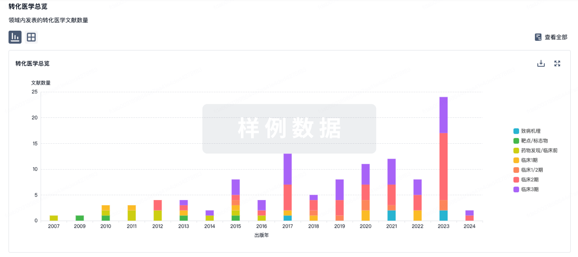
药物交易
使用我们的药物交易数据加速您的研究。
登录
或
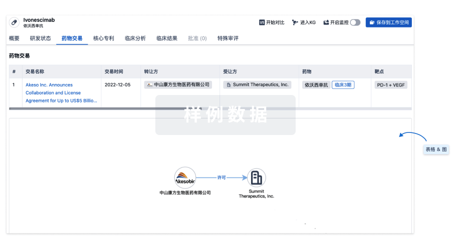
核心专利
使用我们的核心专利数据促进您的研究。
登录
或
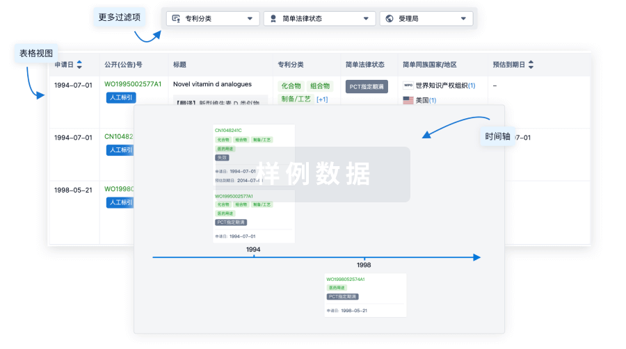
临床分析
紧跟全球注册中心的最新临床试验。
登录
或
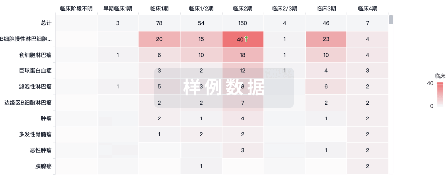
批准
利用最新的监管批准信息加速您的研究。
登录
或
特殊审评
只需点击几下即可了解关键药物信息。
登录
或
芽仔
全新生物医药AI Agent 覆盖科研全链路,让突破性发现快人一步
立即开始免费试用!
智慧芽新药情报库是智慧芽专为生命科学人士构建的基于AI的创新药情报平台,助您全方位提升您的研发与决策效率。
立即开始数据试用!
智慧芽新药库数据也通过智慧芽数据服务平台,以API或者数据包形式对外开放,助您更加充分利用智慧芽新药情报信息。
生物序列数据库
生物药研发创新
免费使用
化学结构数据库
小分子化药研发创新
免费使用